Recipes

While in my day-to-day work I use chessboards and process images of them using the mrgingham chessboard corner detector, this isn't a requirement. In fact, mrcal doesn't care at all where its detections come from. The only requirements on the calibration object are that

• The calibration object is nominally planar; small amounts of deformation are allowed
• The object contains a regular grid of points. Gaps are allowed, but the points that do exist must lie on this grid
• The grid spacing is identical in the horizontal and vertical directions
• Each point in the object is uniquely identifiable in each observation of the object

It's not required that all points are observed in every image of the object: partial observations of the board are supported by mrcal (mrgingham won't detect those, but mrcal has no problem ingesting incomplete views). And boards that don't contain a full grid are supported as well. For instance here's a bug report where somebody used a calibration board with an unrelated fiducial in the middle.

To use a grid detector other than mrgingham, we need to

• produce a compatible corners.vnl file. This is a vnlog (text table) where each row describes a single corner detection
• feed this file to mrcal-calibrate-cameras --corners-cache

A sample corners.vnl describing observations of a toy 2x2 chessboard:

#   filename      x    y  weight
frame0-cam0.jpg 10.2 12.5 1.0   
frame0-cam0.jpg 21.2 15.1 1.0   
frame0-cam0.jpg  9.4 19.5 0.5   
frame0-cam0.jpg 21.3 23.6 1.0   
frame0-cam1.jpg -    -    -     
frame1-cam0.jpg -    -    -     
frame1-cam1.jpg 30.1 39.6 0.25  
frame1-cam1.jpg 45.8 38.5 1.0   
frame1-cam1.jpg -    -    -     
frame1-cam1.jpg 42.5 47.4 1.0   

Whitespace added for clarity. Here we have 2 cameras and 2 frames. Only frame0-cam0.jpg and frame1-cam1.jpg have a chessboard detection, with one of the corners missing in frame1-cam1.jpg.

The corners.vnl file contains 3 or 4 columns. The first 3 columns are:

• filename: a path to the image on disk
• x, y: pixel coordinates of a detected corner in the

If a 4th column is present, it describes the detector's confidence in the detection of that particular corner. It may be either

• level: the decimation level of the detected corner. If the detector needed to cut down the image resolution to find this corner, we report that resolution here. Level-0 means "full-resolution", level-1 means "half-resolution", level-2 means "quarter-resolution" and so on. A level of - or <0 means "skip this point"; this is how incomplete board observations are specified. This "decimation level" interpretation is the mrcal-calibrate-cameras default. This column is reported by mrgingham
• weight: how strongly to weight that corner. More confident detections take stronger weights. This should be inversely proportional to the standard deviation of the detected pixel coordinates. With decimation levels we have \(\mathrm{weight} = 2^{-\mathrm{level}}\). As before, a weight of - or <0 means "skip this point"; this is how incomplete board observations are specified. Select this "weight" interpretation with mrcal-calibrate-cameras --corners-cache-has-weights

If no 4th column is present, we assume an even weight of 1.0 for all the points.

The whole chessboard is described by a sequence of these corner detections, listed in a consistent grid order: the first row is traversed point-by-point in order, then the second row, and so on. Each chessboard image is represented by either exactly \(N_\mathrm{width} N_\mathrm{height}\) corner records or a single record

FILENAME - - -

to represent images with no detected corners. An image with incomplete detections should still contain \(N_\mathrm{width} N_\mathrm{height}\) records in the same consistent order. The missing corners should be given with any x, y, but with \(\mathrm{weight} \leq 0\) or -. The record could also be completely null:

FILENAME - - -

The missing points are treated as outliers by the solver. Currently the diagnostics included these points as outliers as well, although that will likely change in the future.

The mrgingham corner detector is the tool I use to detect corners in images of chessboards (although other methods are available). mrgingham looks for plain chessboards in the images, without any extra fiducials. It reports the corners in the top-most horizontal row in order from left to right. Then the next row down, and the next row, and so on. Here "top", "left" and "right" are the pixel coordinates in the image. The position of each corner in this list uniquely identifies the corner. So the corner in row \(i\), col \(j\) always appears at index \(i N_\mathrm{width} + j\) in the list. This works well, as long as the "horizontal" and "vertical" directions in the image are consistent, which they usually are. However, if the camera orientation isn't identical across cameras or across time, issues can arise.

Consider a 2-camera calibration where one camera is mounted rightside-up, but the other is mounted upside-down. Here the first corner reported in the left camera is the top-left corner in the chessboard, but the first corner reported in the right camera is the bottom-right corner in the chessboard. The first reported corner has index 0, so it must represent the same corner for all cameras, but here it does not.

In the very common situation where the cameras are all mounted right-side-up or sideways or upside-down we can handle this situation by reordering the corners in a mrgingham corners list. This is done by the mrgingham-rotate-corners tool. The usage is simple:

< corners.vnl                        \
mrgingham-rotate-corners [--gridn N] \
  --90  REGEX_CAM_90deg              \
  --180 REGEX_CAM_180deg             \
  --270 REGEX_CAM_270deg             \
  [... more rotation selections ...] \
> corners-rotated.vnl

We pass in the corners.vnl set of detections. Filenames that were captured by a camera rotated by 90deg are selected by REGEX_CAM_90deg and so on. The result is a corners-rotated.vnl with reordered corners that meet the assumptions of the solver, and can be passed to mrcal-calibrate-cameras. Another example:

# camera A is rightside-up
# camera B is mounted sideways
# cameras C,D are upside-down
mrgingham --gridn N                \
  'frame*-cameraA.jpg'             \
  'frame*-cameraB.jpg'             \
  'frame*-cameraC.jpg'             \
  'frame*-cameraD.jpg' |           \
mrgingham-rotate-corners           \
  --gridn N                        \
  --90 cameraB                     \
  --180 'camera[CD]'               \
> corners-rotated.vnl

Usually cameras are calibrated by observing a moving calibration object with stationary cameras. This is not the only possible scheme, and mrcal supports others. A surveyed calibration is one where the poses of the objects being observed are pre-determined (by surveying them, for instance). Then we get a simplified calibration problem:

• Each point in space being observed has a fixed position. This is assumed to be known perfectly
• The camera is stationary, with a non-fixed pose: we solve for it
• Only monocular solves are necessary. Since the objects being observed are fixed, there is no interaction between the multiple cameras being calibrated, and a multi-camera surveyed calibration can be solved by computing several independent monocular calibrations.

Furthermore, it doesn't matter if we're observing chessboards or discrete points or both: everything being observed has a known, fixed position. So when solving these problems we call mrcal.optimize(...) with

• Fixed frames_rt_toref and points arrays localizing the observed objects
• do_optimize_frames = False to tell the optimization to fix them in space

Calibrating in this way is uncommon, so the mrcal-calibrate-cameras tool does not support this directly. But this kind of solve is readily available via the Python APIs, as demonstrated by the test/test-surveyed-calibration.py script:

test/test-surveyed-calibration.py \
  --do-sample                     \
  --make-documentation-plots ''

This script simulates 3 observed chessboards in front of the camera. A long lens is used with a lean lens model (LENSMODEL_OPENCV4). We capture a single frame. The observed image looks like this:

Here we're looking at chessboards, but the observations are given to mrcal as discrete points for flexibility; we could use fixed chessboards identically.

This setup is clearly violating the usual guidelines for capturing calibration data: we have a too-lean lens model, and we're not covering the imager with data. This is still useful to illustrate the processing, however. And this isn't far off from how somebody might capture data for a surveyed calibration.

These kinds of solves usually work off far less data than the usual moving-chessboard calibrations, so they are more susceptible to sampling error causing high projection uncertainty. Fortunately, the techniques that we have for analyzing calibration quality (projection uncertainty quantification and cross-validation differencing) are available here, so we can see how good or bad the results are. Note: today mrcal supports computing the uncertainty of a chessboard-less calibration only if the points are fixed, as they are here; this will be implemented fully in the future.

Similarly to the simulations in the tour of mrcal, we show that the predicted projection uncertainty matches what we get from sampling the input noise multiple times:

We also looked at the effect of input noise on the extrinsics. The error in solved \(z\) in camera coordinates:

Clearly the uncertainty propagation logic is working. Note: today's discrete point handling in mrcal has extra factors that generate this warning when computing an uncertainty:

WARNING: I'm currently treating the point range normalization (penalty) terms as following the same noise model as other measurements. This will bias the uncertainty estimate

This is benign, and the related logic is likely to change in the future.

The usual rule-of-thumb is to gather calibration data at multiple ranges because it is otherwise difficult to disentangle the effects of camera position from the effects of intrinsics. We can demonstrate this explicitly using the same test script: we solve the same calibration problem, with the range to the center chessboard varying.

for z (4 5 8 9 9.5 10 10.5 11 15 20 30) {
    test/test-surveyed-calibration.py \
      --only-report-uncertainty       \
      --range-board 10                \
      --range-board-center $z 2>/dev/null
  } \
| vnl-filter -p z-center,stdev \
| feedgnuplot                \
    --domain                 \
    --vnl                    \
    --autolegend             \
    --y2 'stdev(errz)'       \
    --ymin  0                \
    --y2min 0                \
    --lines                  \
    --points                 \
    --xlabel  'Distance to the middle chessboard (m)' \
    --ylabel  'Reprojection error (pixels)' \
    --y2label 'Position error in z (m)' \
    --legend 'stdev(q)'    'Standard deviation of reprojection at infinity' \
    --legend 'stdev(errz)' 'Standard deviation of the error in z' \
    --title 'Surveyed calibration: effect of camera range variability; 2 cameras at 10m, one variable'

So when all 3 chessboards sit at 10m out, we get far worse uncertainties in both the projection behavior and position estimates defined by the calibration. When running the standard moving-chessboard calibration we have an analogous effect when we consider tilting the chessboard to the camera: chessboard tilt creates the variable ranges required for a well-defined solve.

In our scenario here, the issue is high sampling error causing a high projection uncertainty. One way to mitigate this problem is by gathering more data. Even if everything is stationary, and we capture multiple images of the same stationary scene, we are still capturing multiple samples of the input noise. In theory. If we capture \(N\) times more data, the expected uncertainty improvement is \(\sqrt{N}\). Let's try it by passing the --oversample 10 option:

for z (4 5 8 9 9.5 10 10.5 11 15 20 30) {
    test/test-surveyed-calibration.py \
      --oversample 10                 \
      --only-report-uncertainty       \
      --range-board 10                \
      --range-board-center $z 2>/dev/null
  } \
| vnl-filter -p z-center,stdev \
| feedgnuplot                \
    --domain                 \
    --vnl                    \
    --autolegend             \
    --y2 'stdev(errz)'       \
    --ymin  0                \
    --y2min 0                \
    --lines                  \
    --points                 \
    --xlabel  'Distance to the middle chessboard (m)' \
    --ylabel  'Reprojection error (pixels)' \
    --y2label 'Position error in z (m)' \
    --legend 'stdev(q)'    'Standard deviation of reprojection at infinity' \
    --legend 'stdev(errz)' 'Standard deviation of the error in z' \
    --title 'Surveyed calibration: effect of camera range variability; 2 cameras at 10m, one variable; 10x oversampling'

And it works as expected: we still see the spike, but all the uncertainties are roughly a factor or \(\sqrt{10} = 3.2\) smaller. Note that this works if the input noise is truly gaussian and independent. Empirically, this is mostly true, but may not be 100% true. Techniques that rely heavily on this assumption, such as this one, may not work perfectly in the real world. Take these results with a grain of salt.

When we calibrate a camera system, we're assuming that the physical properties of the system are fixed. If they weren't, then even a very accurate calibration isn't useful: the system may have changed by the time we actually use the computed calibration. We must try to stabilize all parts of the system prior to calibrating, and then we can check to see how well we did.

In the tour of mrcal we used a Samyang 12mm F2.8 fisheye lens. This is not a machine-vision lens; it's intended to be used by human photographers operating an SLR camera. As a result, it has moving parts. In particular, the human-operated focus ring engages an internal mechanism that physically moves the front lens element. Immobilizing the external focus ring does not immobilize the internal mechanism, so any mechanical backlash shows up as an instability in intrinsics.

From experience, I know that this lens is sensitive to mechanical motion, and we can clearly see this in the data. For the tour of mrcal I gathered two independent sets of chessboard images one after another, without moving anything. This was used for cross-validation, and resulted in this diff:

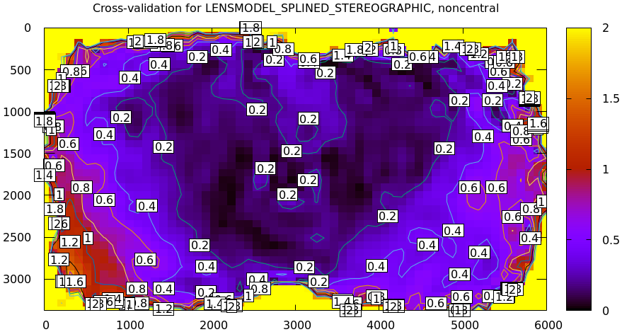
Then I moved the camera and tripod over by 2m or so, and gathered more chessboard images. Comparing these with the previous set showed a clear shift in the intrinsics:

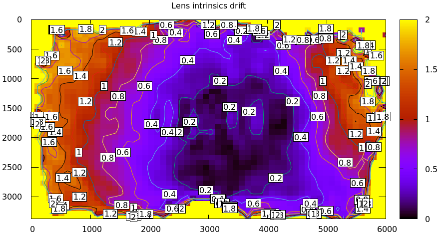
This was from just carefully moving the tripod.

To be clear: this isn't a bad lens, it's just not built with high-accuracy machine vision in mind. A lens intended for machine vision applications would do better. If we had to use this lens, I would gather multiple sets of data before and after stressing the system (shaking, flipping, heating, etc). Then the resulting diffs would tell us how much to trust the calibration.

Similarly to the above discussion about the stability of lens intrinsics, we sometimes want to consider the stability of the camera-camera geometric transformation in a multi-camera system. For instance, it's possible to have a multi-camera system composed of very stable lenses mounted on a not-rigid-enough mount. Any mechanical stresses wouldn't affect the intrinsics, but the extrinsics would shift. Evaluation of this motion is described on the differencing page.

It is often useful to convert a camera model utilizing one lens model to use another one. For instance when using a calibration in an existing system that doesn't support the model we have. This is a common need, so a standalone tool is available for this task: mrcal-convert-lensmodel. Two modes are available:

1. If the given cameramodel file contains optimization_inputs, then we have all the data that was used to compute this model in the first place, and we can re-run the original optimization, using the new lens model. This is the default behavior, and is the preferred choice. However it can only work with models that were computed by mrcal originally.
2. We can sample a grid of points on the imager, unproject them to observation vectors in the camera coordinate system, and then fit a new camera model that reprojects these vectors as closely to the original pixel coordinates as possible. This can be applied to models that didn't come from mrcal. Select this mode by passing --sampled.

Since camera models (lens parameters and geometry) are computed off real pixel observations, the confidence of the projections varies greatly across the imager and across observation distances. The first method uses the original data, so it implicitly respects these uncertainties: uncertain areas in the original model will be uncertain in the new model as well. The second method, however, doesn't have this information: it doesn't know which parts of the imager and space are reliable, so the results suffer.

As always, the intrinsics have some baked-in geometry information. Both methods optimize intrinsics and extrinsics, and output cameramodels with updated versions of both. If --sampled: we can request that only the intrinsics be optimized by passing --intrinsics-only.

Also, if --sampled and not --intrinsics-only: we fit the extrinsics off 3D points, not just observation directions. The distance from the camera to the points is set by --distance. This can take a comma-separated list of distances to use. It's strongly recommended to ask for two different distances:

• A "near" distance: where we expect the intrinsics to have the most accuracy. At the range of the chessboards, usually
• A "far" distance: at "infinity". A few km is good usually.

The reason for this is that --sampled solves at a single distance aren't sufficiently constrained, similar to the issues that result from a surveyed calibration of chessboards all at the same range. If we ask for a single far distance: --distance 1000 for instance, we can easily get an extrinsics shift of 100m. This is aphysical: changing the intrinsics could shift the camera origin by a few mm, but not 100m. Conceptually we want to perform a rotation-only extrinsics solve, but this isn't yet implemented. Passing both a near and far distance appears to constrain the extrinsics well in practice. The computed extrinsics transform is printed on the console, with a warning if an aphysical shift was computed. Do pay attention to the console output.

Some more tool-specific documentation are available in the documentation in mrcal-convert-lensmodel.

Any application that uses camera models is composed of multiple steps, some of which would benefit from mrcal-specific logic. Specifically:

1. For successful long-range triangulation or stereo we need maximum precision in our lens models. mrcal supports LENSMODEL_SPLINED_STEREOGRAPHIC: a rich model that fits real-world lenses better than the lean models used by other tools. This is great, but as of today, mrcal is the only library that knows how to use these models.
2. Furthermore, mrcal can use LENSMODEL_LATLON to describe the rectified system instead of the more traditional LENSMODEL_PINHOLE rectification function. This allows for nice stereo matching even with wide lenses, but once again: these rectified models and images can only be processed with mrcal.

A common need is to use mrcal's improved methods in projects built around legacy stereo processing. This usually means selecting specific chunks of mrcal to utilize, and making sure they can function as part of the existing framework. Some relevant notes follow.

mrcal is primarily a geometric toolkit: after we detect the chessboard corners, we never look at the chessboard images again, and do everything with the detected corner coordinates. This assumes the chessboard detector works perfectly. At least for mrgingham, this is a close-enough assumption; but it's nice to be able to double-check. To do that the mrcal sources include the mrcal-reproject-to-chessboard tool; this is still experimental, so it's not included in a mrcal installation, and currently has to be invoked from source. This tool takes in completed calibration, and reprojects each chessboard image to a chessboard-referenced space: each resulting image shows just the chessboard, with each chessboard corner appearing at exactly the same pixel in each image. Example frame from the tour of mrcal:

analyses/mrcal-reproject-to-chessboard \
  --image-path-prefix images           \
  splined.cameramodel

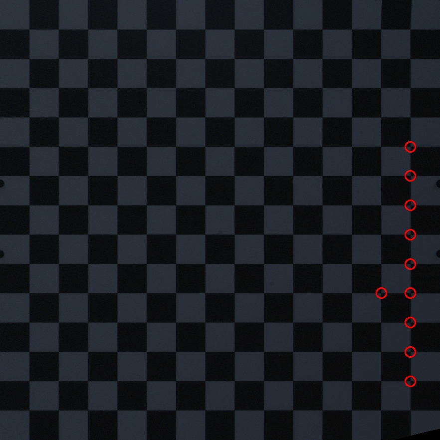
This is a sample frame from the full animation of these images.

The red circles indicate corner observations classified as outliers by the solver. Ideally every reprojected image should be very similar, with each chessboard corner randomly, and independently jumping around a tiny bit (by the amount reported in the fit residuals). If the detector had any issues or an image was faulty in some way, this would be clearly seen by eyeballing the sequence of images. The whole image would shift; or a single non-outlier corner would jump. It's good to eyeball these animations as a final sanity check before accepting a calibration. For questionable calibration objects (such as grids of circles or AprilTags), checking this is essential to discover biases in these implicit detectors.

Ignoring noncentral effects very close to the lens, a camera model maps directions in space to pixel coordinates, with each pixel covering a solid angle of some size. As sensor resolutions increase, the pixels become finer, covering smaller solid angles. For various processing it is often useful to visualize this angular resolution of a camera. For instance to justify using geometric-only techniques, such as the triangulation methods.

mrcal provides the analyses/mrcal-show-model-resolution.py tool to do this. This tool isn't yet "released", so it is not yet part of the installed set, and must be run from the source tree. A sample visualization of the lens from the tour of mrcal:

analyses/mrcal-show-model-resolution.py                        \
  --title "Mean angular resolution (deg/pixel) over the imager" \
  splined.cameramodel

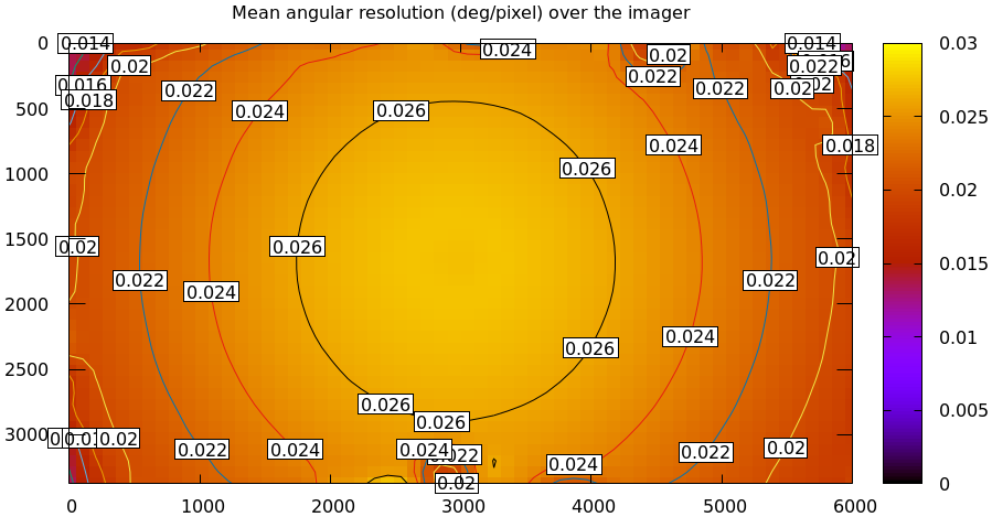
So as we move outwards, each pixel covers less space. Note that at each pixel the projection behavior isn't necessarily isotropic: the resolution may be different if looking in different directions. The current implementation of the tool does assume isotropic behavior, however, and it displays the mean resolution.

Any particular application has requirements for how accurate the mapping and/or localization need to be. Triangulation accuracy scales with the square of range, so performance will be strongly scene-dependent. But we can use mrcal to quickly get a ballpark estimate of how well we can hope to do.

Let's look back at the tour of mrcal. We saw that using LENSMODEL_OPENCV8 was insufficient, and resulted in these projection errors:

mrcal-show-projection-diff \
  --unset key              \
  opencv8.cameramodel      \
  splined.cameramodel

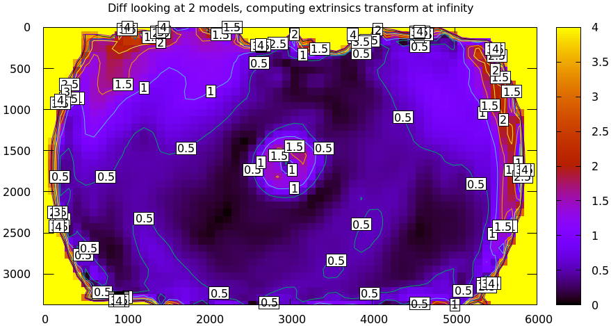
Let's say the lens model error is 0.5 pixels per camera (I'm looking at a rough median of the plots). So at worst, two cameras give us double that: 1.0 pixel error. At worst this applies to disparity directly, so let's assume that.

Noise in stereo matching is usually on the order of 0.3 pixels, so we're going to have on the order of 1.0 + 0.3 = 1.3 pixels of disparity error. Let's see how significant this is. Let's once again go back to tour of mrcal, this time to its stereo matching page. How would 1.3 pixels of disparity error affect that scene? Let's find out.

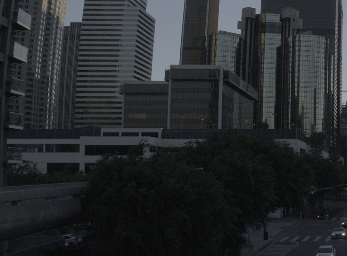
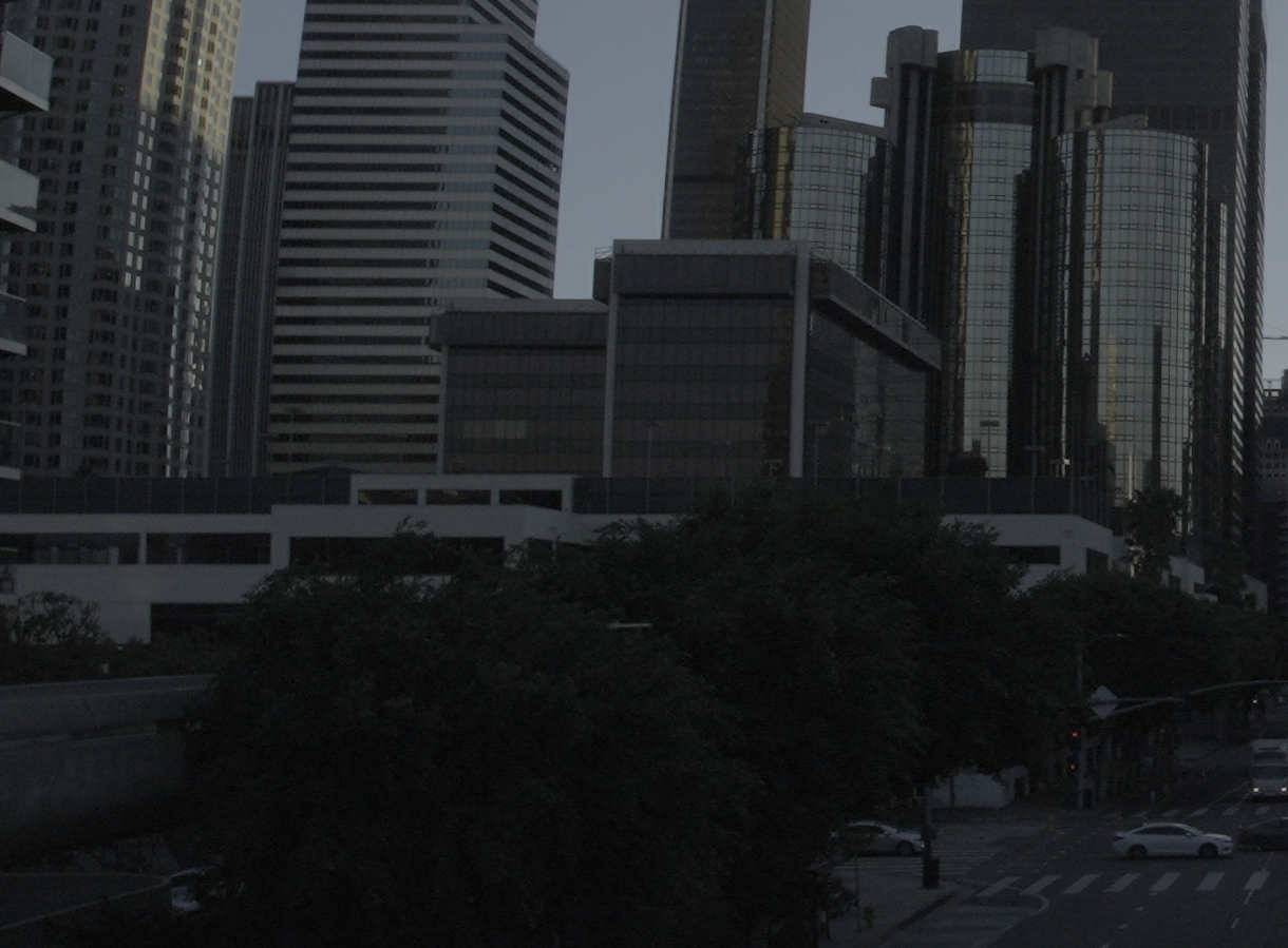
We write a little bit of Python code to rerun the stereo processing, focusing on a section of the scene, for clarity.

#!/usr/bin/python3

import sys
import os
import numpy as np
import numpysane as nps
import mrcal
import cv2
import gnuplotlib as gp

model_filenames = [ f"{i}.cameramodel" for i in (0,1) ]
image_filenames = [ f"{i}.jpg"         for i in (0,1) ]

az_fov_deg = 32.4
el_fov_deg = 24.9
az0_deg    = -20.2
el0_deg    = 6.6

pixels_per_deg                  = -1.
rectification                   = 'LENSMODEL_LATLON'
disp_min,disp_max               = 0,150
range_image_min,range_image_max = 1,1000

disparity_error_expected        = 1.3

models = [mrcal.cameramodel(modelfilename) for modelfilename in model_filenames]

models_rectified = \
    mrcal.rectified_system(models,
                           az_fov_deg          = az_fov_deg,
                           el_fov_deg          = el_fov_deg,
                           az0_deg             = az0_deg,
                           el0_deg             = el0_deg,
                           pixels_per_deg_az   = pixels_per_deg,
                           pixels_per_deg_el   = pixels_per_deg,
                           rectification_model = rectification)

rectification_maps = mrcal.rectification_maps(models, models_rectified)

# This is a hard-coded property of the OpenCV StereoSGBM implementation
disparity_scale = 16

# round to nearest multiple of disparity_scale. The OpenCV StereoSGBM
# implementation requires this
disp_max = disparity_scale*round(disp_max/disparity_scale)
disp_min = disparity_scale*int  (disp_min/disparity_scale)

stereo_sgbm = \
    cv2.StereoSGBM_create(minDisparity      = disp_min,
                          numDisparities    = disp_max - disp_min,
                          blockSize         = 5,
                          P1                = 600,
                          P2                = 2400,
                          disp12MaxDiff     = 1,
                          uniquenessRatio   = 5,
                          speckleWindowSize = 100,
                          speckleRange      = 2 )

images = [mrcal.load_image(f,
                           bits_per_pixel = 24,
                           channels       = 3) for f in image_filenames]

images_rectified = [mrcal.transform_image(images[i],
                                          rectification_maps[i]) \
                    for i in range(2)]

disparity = stereo_sgbm.compute(*images_rectified)

ranges0 = mrcal.stereo_range( disparity,
                              models_rectified,
                              disparity_scale = disparity_scale)

delta = 0.1
ranges1 = mrcal.stereo_range( disparity + delta*disparity_scale,
                              models_rectified,
                              disparity_scale = disparity_scale)

drange_ddisparity = (ranges0-ranges1) / delta

idx_valid = (disparity > 0) * (disparity < 30000)
drange_ddisparity[~idx_valid] = 0

filename_plot = f"{Dout}/sensitivity.png"
title = f"Expected range error assuming disparity error of {disparity_error_expected} pixels"
gp.plot( drange_ddisparity * disparity_error_expected,
         square   = True,
         _set = ('xrange noextend',
                 'yrange reverse noextend',
                 'logscale cb',
                 'cblabel "Expected range error (m)"',
                 'cbtics (.3, 1, 10, 100, 500)'),
         cbrange = [0.3,500],
         _with = 'image',
         tuplesize = 3,
         title     = title)

The rectified images look like this:

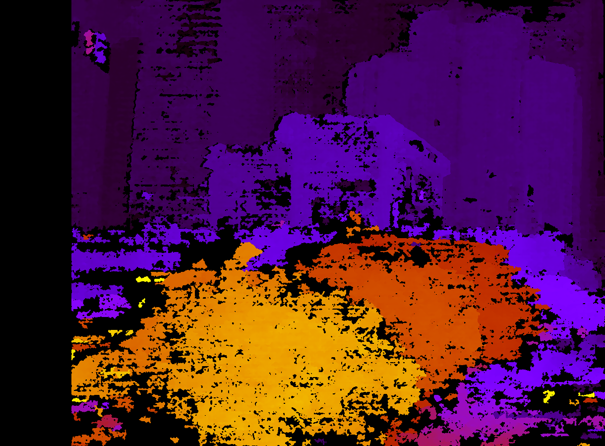
And the disparity image looks like this:

And we compute the range sensitivity. And we plot it:

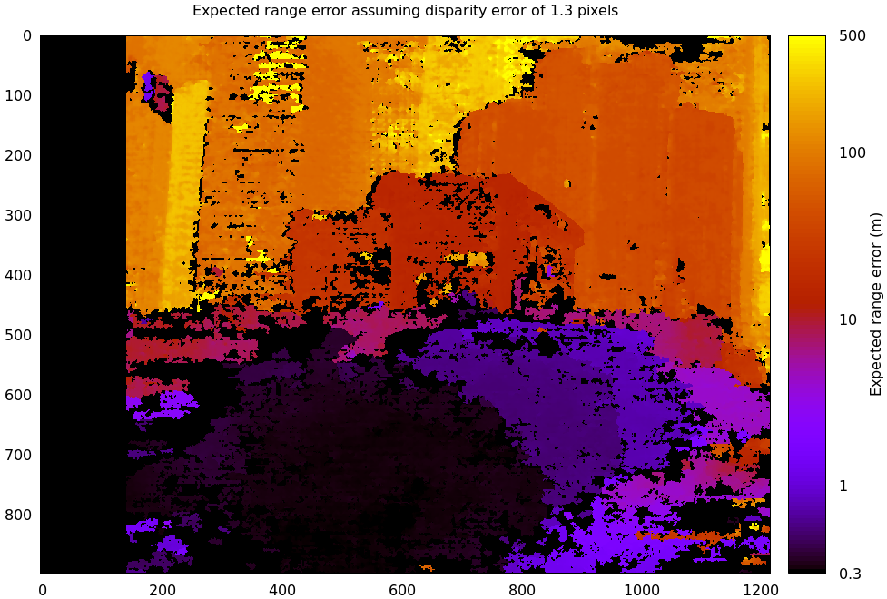
Since triangulation accuracy scales with the square of range, this is a log-scale plot; otherwise it would be illegible. As expected we see that the relatively-nearby tree has an expected range error of < 1m, while the furthest-away building has an expected range error that approaches 500m. Clearly these are rough estimates, but they allow us to quickly gauge the ranging capabilities of a system for a particular scene.