A tour of mrcal: calibration
Table of Contents
The is the first stage in the tour of mrcal.
Gathering chessboard corners
We start by gathering images of a chessboard. I use a large chessboard in order to fill the imager (details about why are on the choreography page). My chessboard has 14x14 internal corners with a corner-corner spacing of 5.88cm. The whole thing is roughly 1m x 1m. A big chessboard such as this is often not completely rigid or completely flat. So I'm using a board backed with 1in of aluminum honeycomb, which addresses these issues: this board is both flat and stable. It took several iterations to settle on this material; see the how-to-calibrate page for details.
An important consideration when gathering calibration images is keeping them in focus. As we shall see later, we want to gather as many close-up images as we can, so depth-of-field is the limiting factor. Moving the focus ring or the aperture ring affects the intrinsics, so ideally a single lens setting can cover both the calibration-time closeups and the working distance (presumably much further out). So for these tests I set the focus to infinity, and gather all my images at F22 to maximize the depth-of-field. To also avoid motion blur I need fast exposures, so I did all the image gathering outside, with bright natural lighting. When gathering real-world calibration data, compromises are often necessary; see the how-to-calibrate page for details.
I gathered some calibration images, and used mrgingham 1.22 to detect the chessboard corners:
mrgingham --jobs 4 --gridn 14 '*.JPG' > corners.vnl
How well did we cover the imager? Did we get the edges and corners?
$ < corners.vnl       \
  vnl-filter -p x,y | \
  feedgnuplot --domain --square --set 'xrange [0:6000] noextend' --set 'yrange [3376:0] noextend'
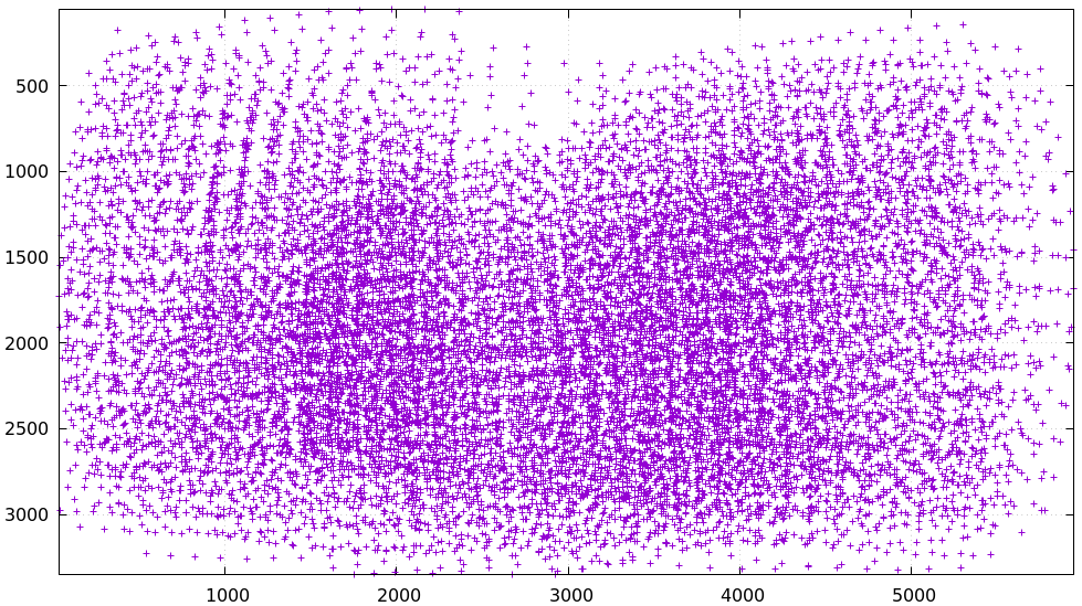
We did OK, except maybe at the top center. This is a good quick/dirty
visualization of calibration data coverage, but as we'll see later, we can do
much better by looking at the projection uncertainty. If we had multiple
cameras, the coverage for each one can be visualized by pre-filtering the
corners.vnl to select specific image filenames. For instance:
< corners.vnl                           \
vnl-filter -p x,y 'filename ~ "left"' | \
feedgnuplot ....
For an arbitrary image we can visualize the corner detections:
$ < corners.vnl head -n5

## generated with mrgingham --jobs 4 --gridn 14 *.JPG
# filename x y level
DSC06041.JPG 781.481013 1476.287623 0
DSC06041.JPG 847.070319 1444.378775 0
DSC06041.JPG 917.514046 1410.696402 0


$ f=DSC06067.JPG

$ < corners.vnl                  \
  vnl-filter                     \
    --perl                       \
    "filename eq \"$f\""         \
    -p x,y,size='2**(1-level)' | \
  feedgnuplot                    \
    --unset key                  \
    --image $f                   \
    --domain                     \
    --square                     \
    --tuplesizeall 3             \
    --with 'points pt 7 ps variable'
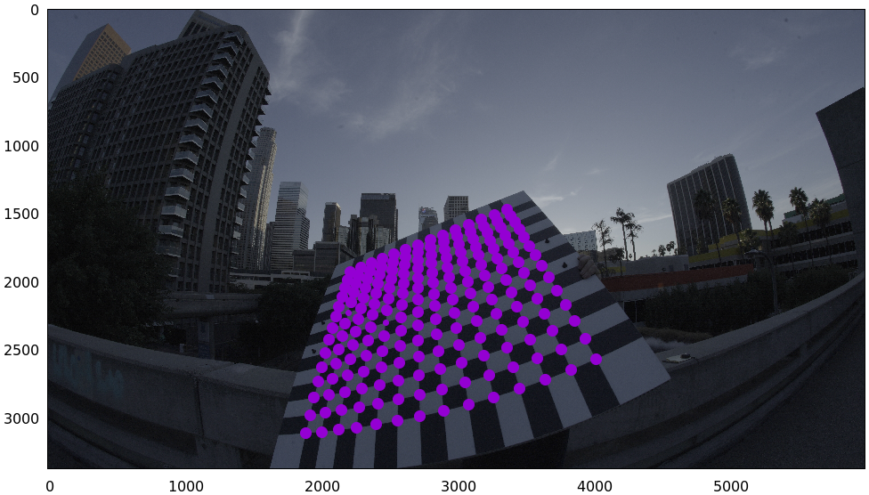
So in this image many of the corners were detected at full-resolution (level-0), but some required downsampling for the detector to find them. This is indicated by smaller circles. The downsampled points have less precision, so they are weighed less in the optimization. How many images produced successful corner detections?
$ < corners.vnl vnl-filter --has x -p filename | uniq | grep -v '#' | wc -l

84
So we have 84 images with detected corners even though we captured 115 images. Most of the misses were probably images where the chessboard wasn't entirely in view, but some could be failures of mrgingham. In any case, 84 observations is usually plenty.
If I had more that one camera, the image filenames would need to indicate what
camera captured each image at which time. I usually name my images
frameFFF-cameraCCC.jpg. Images with the same FFF are assumed to have been
captured at the same instant in time. The exact pattern doesn't matter, but a
constant pattern with a variable FFF and CCC is required.
Monocular calibration with the 8-parameter opencv model
We have data. Let's calibrate. We begin with a lean model used commonly for wide
lenses in other tools: LENSMODEL_OPENCV8. Primarily this works via a rational
radial "distortion" model. Projecting \(\vec p\) in the camera coordinate system:
where \(\vec q\) is the resulting projected pixel, \(k_i\) are the distortion parameters, \(\vec f_{xy}\) is the focal lengths and \(\vec c_{xy}\) is the center pixel of the imager.
Let's compute the calibration using the mrcal-calibrate-cameras tool:
mrcal-calibrate-cameras         \
  --corners-cache corners.vnl   \
  --lensmodel LENSMODEL_OPENCV8 \
  --focal 1900                  \
  --object-spacing 0.0588       \
  --object-width-n 14           \
  '*.JPG'
I'm specifying the initial rough estimate of the focal length (in pixels), the
geometry of my chessboard, the lens model I want to use, chessboard corners we
just detected and the image globs. I have just one camera, so I have one glob:
*.JPG. With more cameras you'd have something like '*-camera0.jpg'
'*-camera1.jpg' '*-camera2.jpg'.
The mrcal-calibrate-cameras tool reports some high-level diagnostics, writes
the output model(s) to disk, and exits:
## initial solve: geometry only
## RMS error: 9.523144801739077

## initial solve: geometry and LENSMODEL_STEREOGRAPHIC core only
=================== optimizing everything except board warp from seeded intrinsics
mrcal.c(5351): Threw out some outliers (have a total of 129 now); going again
...
mrcal.c(5351): Threw out some outliers (have a total of 511 now); going again
## final, full optimization
mrcal.c(5351): Threw out some outliers (have a total of 534 now); going again
mrcal.c(5351): Threw out some outliers (have a total of 553 now); going again
mrcal.c(5351): Threw out some outliers (have a total of 564 now); going again
## RMS error: 0.4120879883977674
RMS reprojection error: 0.4 pixels
Worst residual (by measurement): 1.8 pixels
Noutliers: 564 out of 16464 total points: 3.4% of the data
calobject_warp = [-0.00012726 -0.00014325]

Wrote /tmp/camera-0.cameramodel
The resulting model is available here. This is a mrcal-native .cameramodel
file containing at least the lens parameters and the geometry.
We want to flag down any issues with the data that would violate the assumptions made by the solver. Let's start by sanity-checking the results.
As we can see in the console output, the final RMS reprojection error was 0.4 pixels. Of the 16464 corner observations (84 observations of the board with 14*14 points each), 564 didn't fit the model well-enough, and were thrown out as outliers. The board flex was computed as 0.13mm horizontally, and 0.14mm vertically. That all sounds reasonable.
Let's examine the solution further. We can either
mrcal-calibrate-cameras --explore ...to drop into a REPL after the computation is done. This allows us to look around in the Python session where the solution was computed.- Use the
mrcal-show-...commandline tools on the generatedxxx.cameramodelfiles
The --explore REPL can produce deeper feedback, but the commandline tools are
more convenient, so I here I talk about those.
What does the solve think about our geometry? Does it match reality?
mrcal-show-geometry      \
  opencv8.cameramodel    \
  --show-calobjects      \
  --unset key            \
  --set 'xyplane 0'      \
  --set 'view 80,30,1.5'

Here we see the axes of our camera (purple) situated at the reference coordinate system. In this solve, the camera coordinate system is the reference coordinate system; this would look more interesting with more cameras. In front of the camera (along the \(z\) axis) we can see the solved chessboard poses. There are a whole lot of them, and they're all sitting right in front of the camera with some heavy tilt. This matches with how this chessboard dance was performed: I followed the guidelines of the dance study.
Solve diagnostics
Next, let's examine the residuals more closely. We have an overall RMS reprojection error value from above, but let's look at the full distribution of errors for all the images and cameras:
mrcal-show-residuals    \
  --histogram           \
  --set 'xrange [-2:2]' \
  --unset key           \
  --binwidth 0.1        \
  opencv8.cameramodel

We would like to see a normal distribution (since that's what the noise model assumes), and we roughly do see that here. If the images were captured with varying illumination (which happens with different board orientations and a directional light source), the center cluster or the tails would get over-populated. That would be a violation of the noise model, but things still appear to work OK even in that case.
Let's look deeper. If there's anything really wrong with our data, then we should see it in the worst-fitting images. Let's ask the tool to show us the worst one:
mrcal-show-residuals-board-observation \
  --from-worst                         \
  --vectorscale 200                    \
  --circlescale 0.5                    \
  --set 'cbrange [0:2]'                \
  opencv8.cameramodel                  \
  0
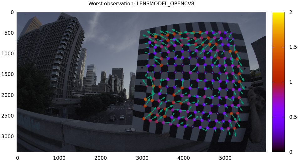
The residual vector for each chessboard corner in this observation is shown, scaled by a factor of 200 for legibility (the actual errors are tiny!) The circle color also indicates the magnitude of the errors. The size of each circle represents the weight given to that point. The weight is reduced for points that were detected at a lower resolution by the chessboard detector. So even high reprojection errors (shown as the vectors) could result in low measurements if the weight was low. Points thrown out as outliers are not shown at all.
Residual plots such as this one are a good way to identify common data-gathering issues such as:
- out-of focus images
- images with motion blur
- rolling shutter effects
- camera synchronization errors
- chessboard detector failures
- insufficiently-rich models (of the lens or of the chessboard shape or anything else)
See the how-to-calibrate page for practical details. Back to this image. In absolute terms, even this worst-fitting image fits really well. The RMS reprojection error in this image is 0.70 pixels. The residuals in this image look mostly reasonable, but there is an issue: if the model fit this data well, the residuals would sample independent, random noise. Thus the residuals would all be uncorrelated with each other, but here there's a pattern: we can see that the errors are mostly radial in the chessboard (they point to/from the center). A unmodeled chessboard flex could cause this kind of problem, for instance. This is a source of bias in this solution. Let's keep going, keeping this in mind.
One issue with lean models such as LENSMODEL_OPENCV8 (used here) is that the
radial distortion is never quite right, especially as we move further and
further away from the optical axis: this is the last point in the common-errors
list above. The result of these radial distortion errors is high residuals in
the corners and near the edges of the image. We can clearly see this here in the
10th-worst image (10th worst and not the worst because the really
poor-fitting points are thrown out as outliers):
mrcal-show-residuals-board-observation \
  --from-worst                         \
  --vectorscale 200                    \
  --circlescale 0.5                    \
  --set 'cbrange [0:2]'                \
  opencv8.cameramodel                  \
  10
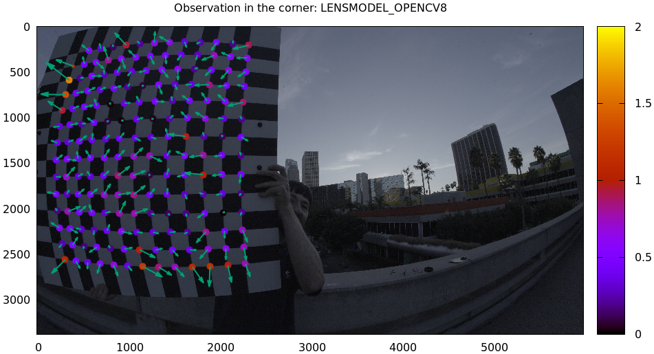
Clearly this image is a problem: the points near the corners have poor residuals, and the entire column of points at the edge was thrown out as outliers. We note that this is observation 47, so that we can come back to it later.
And we can see this same high-error-in-the-corners effect in the residual magnitudes of all the observations:
mrcal-show-residuals                   \
  --magnitudes                         \
  --set 'cbrange [0:1.5]'              \
  opencv8.cameramodel
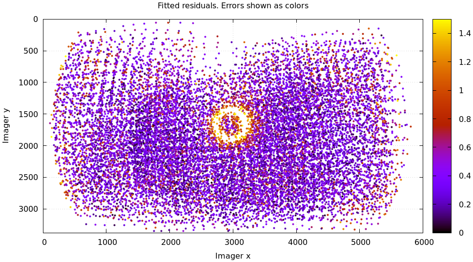
In addition to the expected high errors at the edges, this plot also shows an anomalous ring of poorly-fitting observations at the center. This could maybe be caused by the solver sacrificing accuracy at the center of the image to get a better fit in the much larger areas further out? We shall see in a bit. Let's look at the systematic errors in another way: let's look at all the residuals over all the observations, color-coded by their direction, ignoring the magnitudes:
mrcal-show-residuals    \
  --directions          \
  --unset key           \
  opencv8.cameramodel
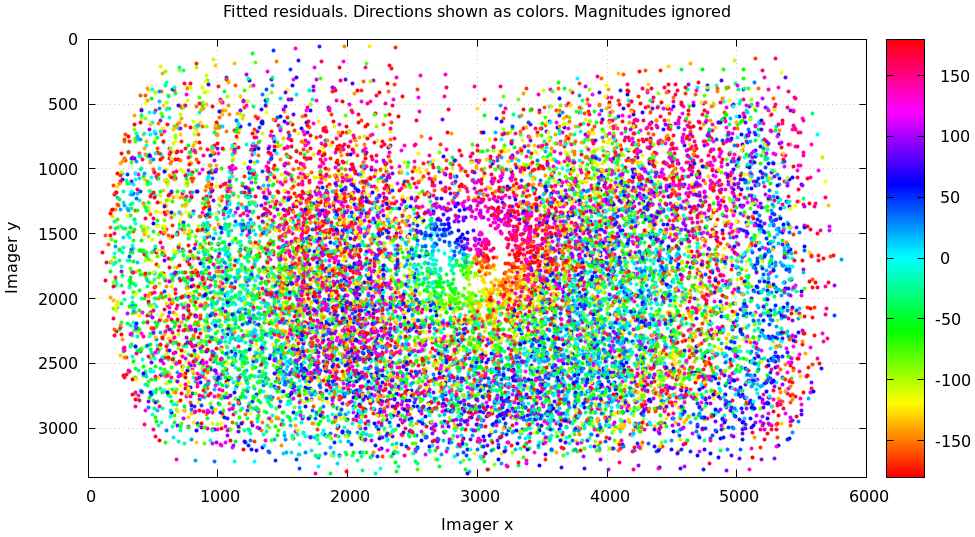
As before, if the model fit the observations, the errors would represent random noise, and no color pattern would be discernible in these dots. But here we can clearly see the colors clustered together. This is not random noise, and is a very clear indication that this lens model is not able to fit this data.
It would be good to have a quantitative measure of these systematic patterns. At this time mrcal doesn't provide an automated way to do that. This will be added in the future.
Clearly there're unmodeled errors in this solve. As we have seen, the errors here are all fairly small, but they become important when doing precision work like, for instance, long-range stereo.
Let's fix it.
Monocular calibration with a splined stereographic model
Usable uncertainty quantification and accurate projections are major goals of mrcal. To achive these, mrcal supports a splined stereographic model, briefly summarized below. We use this splined stereographic model to more precisely model the behavior or this lens.
Splined stereographic model definition
The base of a splined stereographic model is a stereographic projection. In this projection, a point that lies an angle \(\theta\) off the camera's optical axis projects to \(\left|\vec q - \vec q_\mathrm{center}\right| = 2 f \tan \frac{\theta}{2}\) pixels from the imager center, where \(f\) is the focal length. Note that this representation supports projections behind the camera (\(\theta > 90^\circ\)) with a single singularity directly behind the camera. This is unlike the pinhole model, which has \(\left|\vec q - \vec q_\mathrm{center}\right| = f \tan \theta\), and projects to infinity as \(\theta \rightarrow 90^\circ\). The pinhole model can not represent projections behind the imager.
Basing the new model on a stereographic projection lifts the inherent
forward-view-only limitation of LENSMODEL_OPENCV8.
Let \(\vec p\) be the camera-coordinate system point being projected. The angle off the optical axis is
\[ \theta \equiv \tan^{-1} \frac{\left| \vec p_{xy} \right|}{p_z} \]
The normalized stereographic projection is
\[ \vec u \equiv \frac{\vec p_{xy}}{\left| \vec p_{xy} \right|} 2 \tan\frac{\theta}{2} \]
This initial projection operation unambiguously collapses the 3D point \(\vec p\) into a 2D vector \(\vec u\). We then use \(\vec u\) to look-up an adjustment factor \(\Delta \vec u\) using two splined surfaces: one for each of the two elements:
\[ \Delta \vec u \equiv \left[ \begin{aligned} \Delta u_x \left( \vec u \right) \\ \Delta u_y \left( \vec u \right) \end{aligned} \right] \]
We can then define the rest of the projection function:
\[\vec q = \left[ \begin{aligned} f_x \left( u_x + \Delta u_x \right) + c_x \\ f_y \left( u_y + \Delta u_y \right) + c_y \end{aligned} \right] \]
The parameters we can optimize are the spline control points and \(f_x\), \(f_y\), \(c_x\) and \(c_y\), the usual focal-length-in-pixels and imager-center values.
Solving
Let's run the same exact calibration as before, but using the richer model to specify the lens:
mrcal-calibrate-cameras                                                         \
  --corners-cache corners.vnl                                                   \
  --lensmodel LENSMODEL_SPLINED_STEREOGRAPHIC_order=3_Nx=30_Ny=18_fov_x_deg=150 \
  --focal 1900                                                                  \
  --object-spacing 0.0588                                                       \
  --object-width-n 14                                                           \
  '*.JPG'
Reported diagnostics:
## initial solve: geometry only
## RMS error: 9.523144801739077

## initial solve: geometry and LENSMODEL_STEREOGRAPHIC core only
=================== optimizing everything except board warp from seeded intrinsics
mrcal.c(5351): Threw out some outliers (have a total of 28 now); going again
## final, full optimization
## RMS error: 0.24540598163794722
RMS reprojection error: 0.2 pixels
Worst residual (by measurement): 1.3 pixels
Noutliers: 28 out of 16464 total points: 0.2% of the data
calobject_warp = [-1.26851438e-04 -8.03269701e-05]

Wrote /tmp/camera-0.cameramodel
The resulting model is available here.
The requested lens model
LENSMODEL_SPLINED_STEREOGRAPHIC_order=3_Nx=30_Ny=18_fov_x_deg=150 is the only
difference in the command. Unlike LENSMODEL_OPENCV8, this model has some
configuration parameters: the spline order (we use cubic splines here), the
spline density (here each spline surface has 30 x 18 knots), and the rough
horizontal field-of-view we support (we specify about 150 degrees horizontal
field of view). These parameters are fixed in the model, and are not subject to
optimization.
There're over 1000 lens parameters here, but the problem is sparse, so we can still process this in a reasonable amount of time.
The previous LENSMODEL_OPENCV8 solve had 564 points that fit so poorly, the
solver threw them away as outliers; here we have only 28. The RMS reprojection
error dropped from 0.4 pixels to 0.2 pixels. The estimated chessboard shape
stayed roughly the same: flat. These are all what we expect and hope to see.
Let's look at the residual distribution in this solve, compared to before:
mrcal-show-residuals    \
  --histogram           \
  --set 'xrange [-2:2]' \
  --unset key           \
  --binwidth 0.1        \
  splined.cameramodel
This still has the nice bell curve, but the residuals are lower: the data fits better than before.
Let's look at the worst-fitting single image:
mrcal-show-residuals-board-observation \
  --from-worst                         \
  --vectorscale 200                    \
  --circlescale 0.5                    \
  --set 'cbrange [0:2]'                \
  splined.cameramodel                  \
  0
Interestingly, the worst observation here is the same one we saw with
LENSMODEL_OPENCV8, so we can do a nice side-by-side comparison:
All the errors are significantly smaller. The previous radial pattern is still there, but is much less pronounced.
What happens when we look at the image that showed a poor fit in the corner previously? It was observation 47.
mrcal-show-residuals-board-observation \
  --vectorscale 200                    \
  --circlescale 0.5                    \
  --set 'cbrange [0:2]'                \
  splined.cameramodel                  \
  47
And the residual magnitudes of all the observations:
mrcal-show-residuals                   \
  --magnitudes                         \
  --set 'cbrange [0:1.5]'              \
  splined.cameramodel
Neat! The model fits the data at the edges now. And what about the residual directions?
mrcal-show-residuals    \
  --directions          \
  --unset key           \
  splined.cameramodel
Much better than before: the color clustering is gone. The poorly-fitting
ring in the center is still there, but it is being modeled by this splined model
far better than how LENSMODEL_OPENCV8 did (error magnitudes are much better).
We do still see a clear pattern in the directions inside the ring, so it could
still be improved: a denser spline spacing would do better. This is a peculiar
image processing artifact of the Sony Alpha 7 III camera: from experience, other
cameras using this lens do not exhibit this effect. See the tour of mrcal 2.2
for instance; this used the same lens with a different camera.
We can also visualize the magnitude of the vector field defined by the splined surfaces \(\left| \Delta \vec u \right|\):
mrcal-show-splined-model-correction   \
  --set 'cbrange [0:0.1]'             \
  --unset grid                        \
  --set 'xrange [:] noextend'         \
  --set 'yrange [:] noextend reverse' \
  --set 'key opaque box'              \
  splined.cameramodel
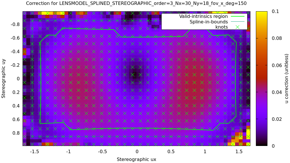
Each X in the plot is a "knot" of the spline surface, a point where a control point value is defined. We're looking at the spline domain, so the axes of the plot are the normalized stereographic projection coordinates \(u_x\) and \(u_y\), and the knots are arranged in a regular grid. The region where the spline surface is well-defined begins at the 2nd knot from the edges; its boundary is shown as a thin green line. The valid-intrinsics region (the area where the intrinsics are confident because we had sufficient chessboard observations there) is shown as a thick, green curve. Since each \(\vec u\) projects to a pixel coordinate \(\vec q\) in some nonlinear way, this curve is not straight.
We want the valid-intrinsics region to lie entirely within the spline-in-bounds region, and we get that here nicely. If some observations did lie outside the spline-in-bounds regions, the projection behavior there would be less flexible than the rest of the model, resulting in less realistic uncertainties, and a larger-fov splined model would be more appropriate. See the lensmodel documentation for more detail.
Alternately, I can look at the spline surface as a function of the pixel coordinates:
mrcal-show-splined-model-correction   \
  --set 'cbrange [0:0.1]'             \
  --imager-domain                     \
  --unset grid                        \
  --set 'xrange [:] noextend'         \
  --set 'yrange [:] noextend reverse' \
  --set 'key opaque box'              \
  splined.cameramodel
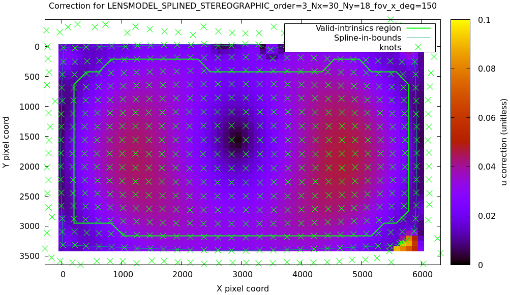
Now the valid-intrinsics region is straight, but the spline-in-bounds region is a curve. Projection at the edges is poorly-defined, so the boundary of the spline-in-bounds region appears irregular in this view.
I can also look at the correction vector field:
mrcal-show-splined-model-correction \
  --vectorfield                     \
  --imager-domain                   \
  --unset grid                      \
  --set 'xrange [-300:6300]'        \
  --set 'yrange [3676:-300]'        \
  --set 'key opaque box'            \
  --gridn 40 30                     \
  splined.cameramodel

This doesn't show anything noteworthy in this solve, but seeing it can be informative with other lenses.
Next
Now we can compare the calibrated models.