A tour of mrcal: calibration
Table of Contents
The is the first stage in the tour of mrcal.
Gathering chessboard corners
We start by gathering images of a chessboard. This is a wide lens, so I need a large chessboard in order to fill the imager. My chessboard has 10x10 internal corners with a corner-corner spacing of 7.7cm. A big chessboard such as this is never completely rigid or completely flat. I'm using a board backed with 2cm of foam, which keeps the shape stable over short periods of time, long-enough to complete a board dance. But the shape still drifts with changes in temperature and humidity, so mrcal estimates the board shape as part of its calibration solve.
An important consideration when gathering calibration images is keeping them in focus. As we shall see later, we want to gather as many close-up images as we can, so depth-of-field is the limiting factor. Moving the focus ring or the aperture ring on the lens may affect the intrinsics, so ideally a single lens setting can cover both the calibration-time closeups and the working distance (presumably much further out).
So for these tests I set the focus to infinity, and gather all my images at F22 to maximize the depth-of-field. To also avoid motion blur I need fast exposures, so I did all the image gathering outside, with bright natural lighting.
The images live here. I'm using mrgingham 1.19 to detect the chessboard corners:
mrgingham -j3 '*.JPG' > corners.vnl
How well did we cover the imager? Did we get the edges and corners?
$ < corners.vnl       \
  vnl-filter -p x,y | \
  feedgnuplot --domain --square --set 'xrange [0:6016]' --set 'yrange [4016:0]'
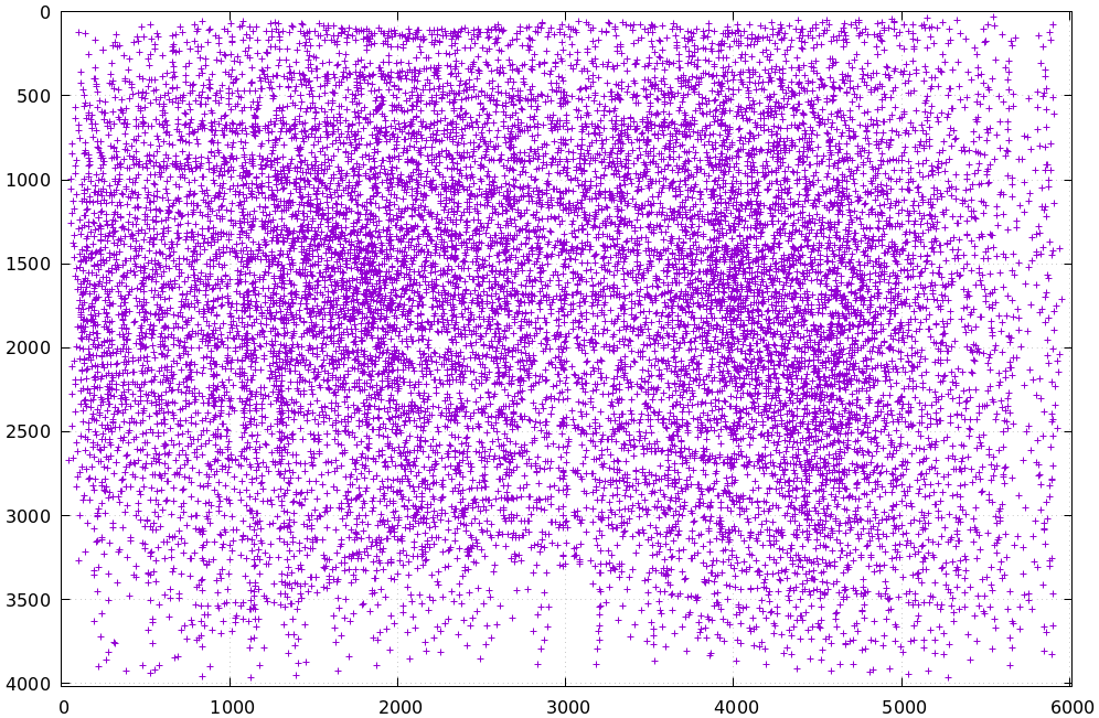
Looks like we did OK. It's a bit thin along the bottom edge, but not terrible. Visualizing the observations in this way is interesting but not necessary, since thin observations will clearly result in poor projection uncertainty we can automatically detect; much more on that later.
For an arbitrary image we can visualize at the corner detections:
$ < corners.vnl head -n5

## generated with mrgingham -j3 *.JPG
# filename x y level
DSC_7305.JPG 3752.349000 168.802000 2
DSC_7305.JPG 3844.411234 150.264910 0
DSC_7305.JPG 3950.404000 132.480000 2


$ f=DSC_7305.JPG

$ < corners.vnl                  \
  vnl-filter                     \
    --perl                       \
    "filename eq \"$f\""         \
    -p x,y,size='2**(1-level)' | \
  feedgnuplot                    \
    --image $f                   \
    --domain                     \
    --square                     \
    --tuplesizeall 3             \
    --with 'points pt 7 ps variable'
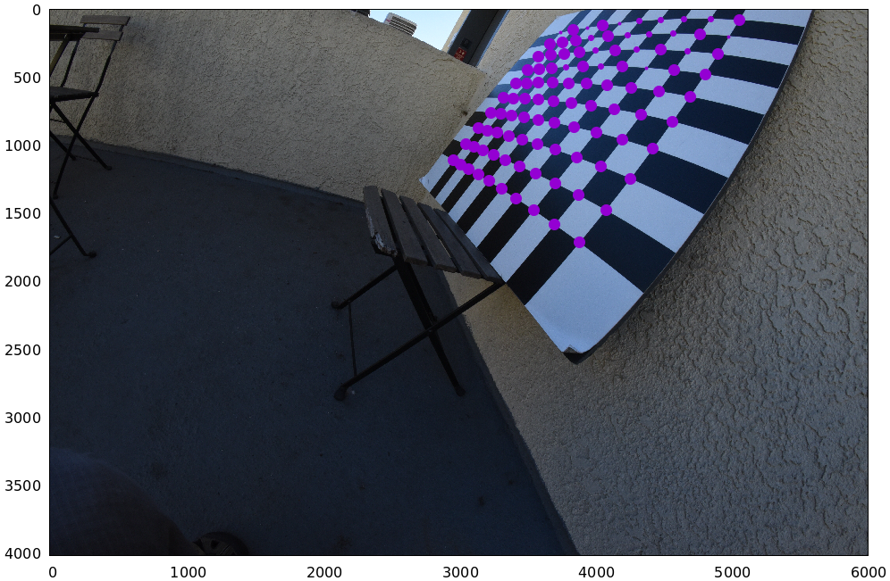
So in this image many of the corners were detected at full-resolution (level-0), but some required downsampling for the detector to find them. This is indicated by smaller circles. The downsampled points have less precision, so they are weighed less in the optimization. How many images produced successful corner detections?
$ < corners.vnl vnl-filter --has x -p filename | uniq | grep -v '#' | wc -l

161
So we have 161 images with detected corners. Most of the misses are probably images where the chessboard wasn't entirely in view, but some could be failures of mrgingham. In any case, 161 observations is plenty.
If I had more that one camera, the image filenames would need to indicate what
camera captured each image at which time. I generally use
frameFFF-cameraCCC.jpg. Images with the same FFF are assumed to have been
captured at the same instant in time.
Monocular calibration with the 8-parameter opencv model
Let's calibrate the intrinsics! We begin with LENSMODEL_OPENCV8, a lean model
that supports wide lenses decently well. Primarily it does this with a rational
radial "distortion" model. Projecting \(\vec p\) in the camera coordinate system:
Where \(\vec q\) is the resulting projected pixel, \(\vec f_{xy}\) is the focal lengths and \(\vec c_{xy}\) is the center pixel of the imager.
Let's compute the calibration using the mrcal-calibrate-cameras tool:
mrcal-calibrate-cameras         \
  --corners-cache corners.vnl   \
  --lensmodel LENSMODEL_OPENCV8 \
  --focal 1700                  \
  --object-spacing 0.077        \
  --object-width-n 10           \
  '*.JPG'
I'm specifying the initial very rough estimate of the focal length (in pixels),
the geometry of my chessboard (10x10 board with 0.077m spacing between corners),
the lens model I want to use, chessboard corners we just detected, the estimated
uncertainty of the corner detections (more on this later) and the image globs. I
have just one camera, so I have one glob: *.JPG. With more cameras you'd have
something like '*-camera0.jpg' '*-camera1.jpg' '*-camera2.jpg'.
We could pass --explore to drop into a REPL after the computation is done, so
that we can look around. The most common diagnostic images can be made by
running the mrcal-show-... commandline tools on the generated
xxx.cameramodel files, but --explore can be useful to get more sophisticated
feedback.
The mrcal-calibrate-cameras tool reports some high-level diagnostics, writes
the output model(s) to disk, and exits:
## initial solve: geometry only
## RMS error: 31.606057232034026

## initial solve: geometry and LENSMODEL_STEREOGRAPHIC core only
=================== optimizing everything except board warp from seeded intrinsics
mrcal.c(5355): Threw out some outliers (have a total of 53 now); going again
mrcal.c(5355): Threw out some outliers (have a total of 78 now); going again
## final, full optimization
mrcal.c(5355): Threw out some outliers (have a total of 155 now); going again
## RMS error: 0.7086476918204073
RMS reprojection error: 0.7 pixels
Worst residual (by measurement): 6.0 pixels
Noutliers: 155 out of 16100 total points: 1.0% of the data
calobject_warp = [-0.00104306  0.00051718]

Wrote ./camera-0.cameramodel
The resulting model is renamed to opencv8.cameramodel, and is available here.
This is a mrcal-native .cameramodel file containing at least the lens
parameters and the geometry.
Let's sanity-check the results. We want to flag down any issues with the data that would violate the assumptions made by the solver.
The tool reports some diagnostics. As we can see, the final RMS reprojection error was 0.7 pixels. Of the 16100 corner observations (161 observations of the board with 10*10 = 100 points each), 155 didn't fit the model well-enough, and were thrown out as outliers. And the board flex was computed as 1.0mm horizontally, and 0.5mm vertically in the opposite direction. That all sounds reasonable.
What does the solve think about our geometry? Does it match reality?
mrcal-show-geometry      \
  opencv8.cameramodel    \
  --show-calobjects      \
  --unset key            \
  --set 'xyplane 0'      \
  --set 'view 80,30,1.5'

Here we see the axes of our camera (purple) situated at the reference coordinate system. In this solve, the camera coordinate system is the reference coordinate system; this would look more interesting with more cameras. In front of the camera (along the \(z\) axis) we can see the solved chessboard poses. There are a whole lot of them, and they're all sitting right in front of the camera with some heavy tilt. This matches with how this chessboard dance was performed (by following the guidelines set by the dance study).
Next, let's examine the residuals more closely. We have an overall RMS reprojection error value from above, but let's look at the full distribution of errors for all the cameras:
mrcal-show-residuals    \
  --histogram           \
  --set 'xrange [-4:4]' \
  --unset key           \
  --binwidth 0.1        \
  opencv8.cameramodel

We would like to see a normal distribution since that's what the noise model assumes. We do see this somewhat, but the central cluster is a bit over-populated. This is a violation of the noise model, bit it's normal-ish, and there isn't a whole lot I can do about it, so I will claim this is close-enough. A common cause of such distributions is observing corners with different intensities; this happens all the time as the angle to the illumination source changes.
Let's look deeper. If there's anything really wrong with our data, then we should see it in the worst-fitting images. Let's ask the tool to see the worst image:
mrcal-show-residuals-board-observation \
  --from-worst                         \
  --vectorscale 100                    \
  --circlescale 0.5                    \
  --set 'cbrange [0:3]'                \
  opencv8.cameramodel                  \
  0
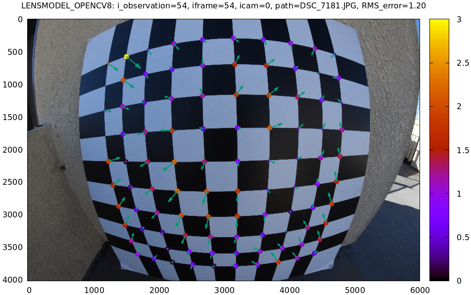
The residual vector for each chessboard corner in this observation is shown, scaled by a factor of 100 for legibility (the actual errors are tiny!) The circle color also indicates the magnitude of the errors. The size of each circle represents the weight given to that point. The weight is reduced for points that were detected at a lower resolution by the chessboard detector. Points thrown out as outliers are not shown at all.
Residual plots such as this one are a good way to identify common data-gathering issues such as:
- out-of focus images
- images with motion blur
- rolling shutter effects
- synchronization errors
- chessboard detector failures
- insufficiently-rich models (of the lens or of the chessboard shape or anything else)
Back to this image. In absolute terms, even this worst-fitting image fits really well. The RMS error of the errors in this image is 1.20 pixels. The residuals in this image look mostly reasonable. There is a pattern, however: the errors are mostly radial (point to/from the center). This could cause biases later on. Let's keep going, keeping this in mind as something we should address later.
One issue with lean models such as LENSMODEL_OPENCV8, which is used here, is
that the radial distortion is never quite right, especially as we move further
and further away from the optical axis: this is the last point in the
common-errors list above. The result of these radial distortion errors is high
residuals in the corners of the image. We can clearly see this here in the
3rd-worst image:
mrcal-show-residuals-board-observation \
  --from-worst                         \
  --vectorscale 100                    \
  --circlescale 0.5                    \
  --set 'cbrange [0:3]'                \
  opencv8.cameramodel                  \
  2
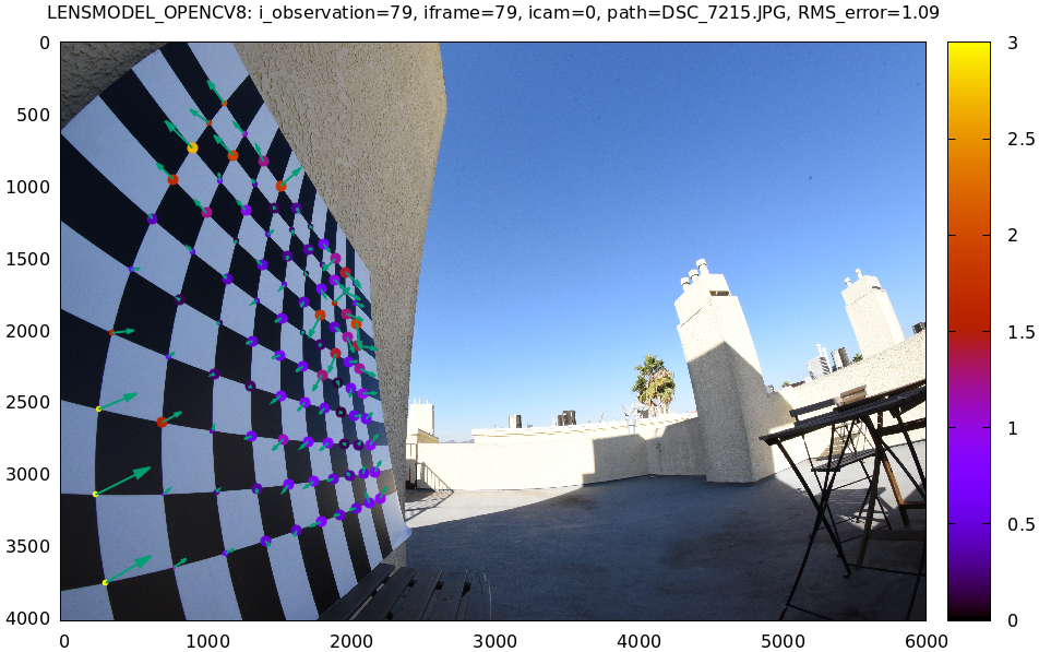
This is clearly a problem. We note that we looked at observation 79, so that we can come back to it later.
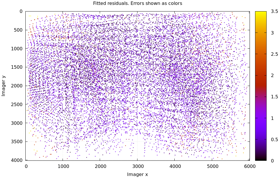
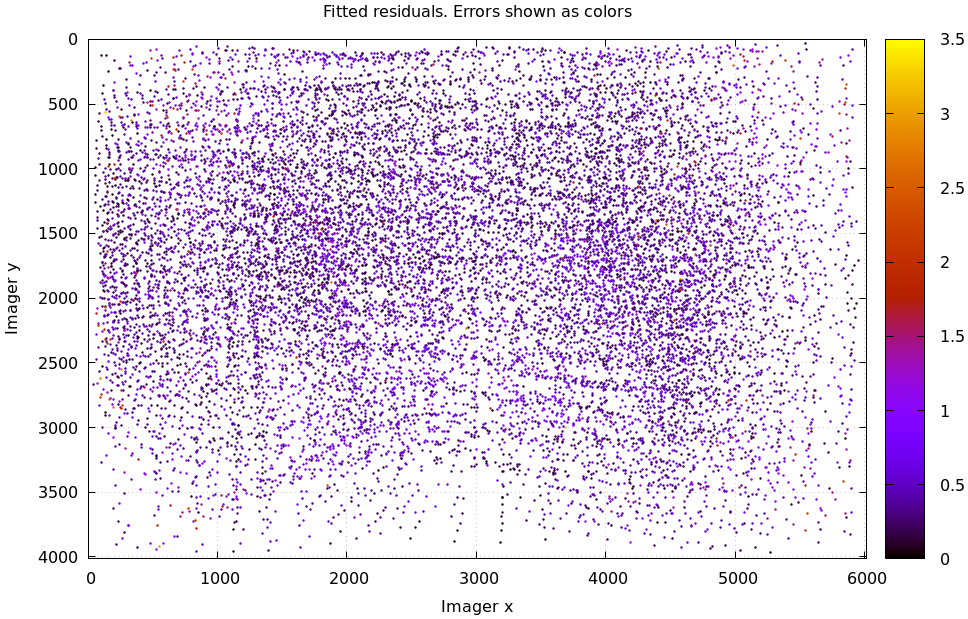
And we can see this same high-error-in-the-corners effect in the residual magnitudes of all the observations:
mrcal-show-residuals                   \
  --magnitudes                         \
  --set 'cbrange [0:3.5]'              \
  opencv8.cameramodel
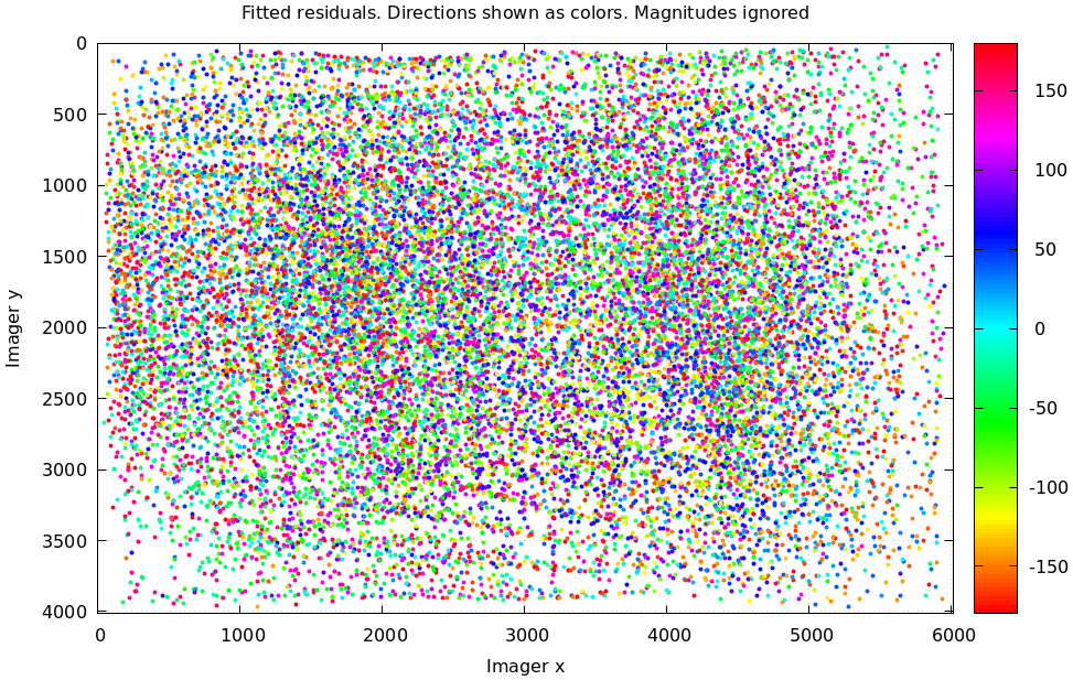
Let's look at the systematic errors in another way: let's look at all the residuals over all the observations, color-coded by their direction, ignoring the magnitudes:
mrcal-show-residuals    \
  --directions          \
  --unset key           \
  opencv8.cameramodel
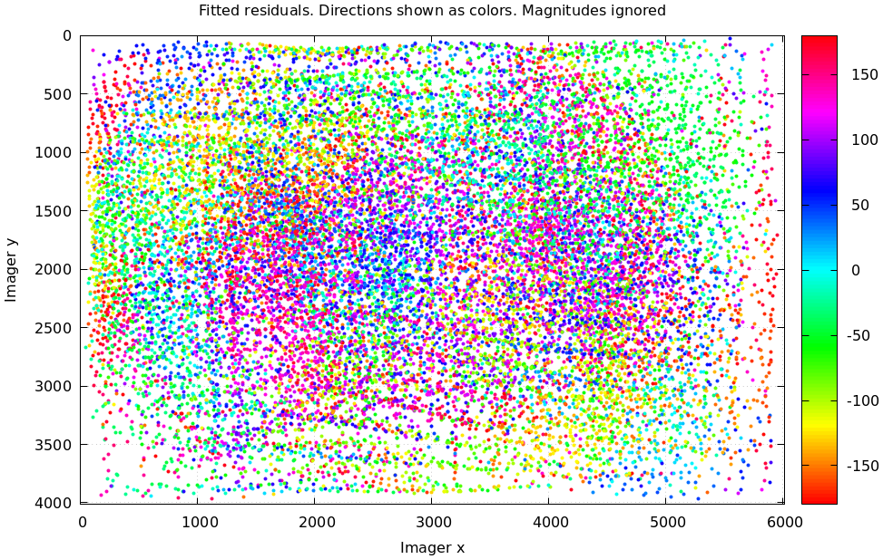
As before, if the model fit the observations, the errors would represent random noise, and no color pattern would be discernible in these dots. Here we can clearly see lots of green in the top-right and top and left, lots of blue and magenta in the center, yellow at the bottom, and so on. This is not random noise, and is a very clear indication that this lens model is not able to fit this data.
It would be good to have a quantitative measure of these systematic patterns. At this time mrcal doesn't provide an automated way to do that. This will be added in the future.
Clearly there're unmodeled errors in this solve. As we have seen, the errors here are all fairly small, but they become very important when doing precision work like, for instance, long-range stereo.
Let's fix it.
Monocular calibration with a splined stereographic model
Usable uncertainty quantification and accurate projections are major goals of mrcal. To achive these, mrcal supports a splined stereographic model, described in detail here.
Splined stereographic model definition
The basis of a splined stereographic model is a stereographic projection. In this projection, a point that lies an angle \(\theta\) off the camera's optical axis projects to \(\left|\vec q - \vec q_\mathrm{center}\right| = 2 f \tan \frac{\theta}{2}\) pixels from the imager center, where \(f\) is the focal length. Note that this representation supports projections behind the camera (\(\theta > 90^\circ\)) with a single singularity directly behind the camera. This is unlike the pinhole model, which has \(\left|\vec q - \vec q_\mathrm{center}\right| = f \tan \theta\), and projects to infinity as \(\theta \rightarrow 90^\circ\).
Basing the new model on a stereographic projection lifts the inherent
forward-view-only limitation of LENSMODEL_OPENCV8. To give the model enough
flexibility to be able to represent any projection function, I define two
correction surfaces.
Let \(\vec p\) be the camera-coordinate system point being projected. The angle off the optical axis is
\[ \theta \equiv \tan^{-1} \frac{\left| \vec p_{xy} \right|}{p_z} \]
The normalized stereographic projection is
\[ \vec u \equiv \frac{\vec p_{xy}}{\left| \vec p_{xy} \right|} 2 \tan\frac{\theta}{2} \]
This initial projection operation unambiguously collapses the 3D point \(\vec p\) into a 2D point \(\vec u\). We then use \(\vec u\) to look-up an adjustment factor \(\Delta \vec u\) using two splined surfaces: one for each of the two elements of
\[ \Delta \vec u \equiv \left[ \begin{aligned} \Delta u_x \left( \vec u \right) \\ \Delta u_y \left( \vec u \right) \end{aligned} \right] \]
We can then define the rest of the projection function:
\[\vec q = \left[ \begin{aligned} f_x \left( u_x + \Delta u_x \right) + c_x \\ f_y \left( u_y + \Delta u_y \right) + c_y \end{aligned} \right] \]
The parameters we can optimize are the spline control points and \(f_x\), \(f_y\), \(c_x\) and \(c_y\), the usual focal-length-in-pixels and imager-center values.
Solving
Let's run the same exact calibration as before, but using the richer model to specify the lens:
mrcal-calibrate-cameras                                                         \
  --corners-cache corners.vnl                                                   \
  --lensmodel LENSMODEL_SPLINED_STEREOGRAPHIC_order=3_Nx=30_Ny=20_fov_x_deg=150 \
  --focal 1700                                                                  \
  --object-spacing 0.077                                                        \
  --object-width-n 10                                                           \
  '*.JPG'
Reported diagnostics:
## initial solve: geometry only
## RMS error: 31.606057232034026

## initial solve: geometry and LENSMODEL_STEREOGRAPHIC core only
=================== optimizing everything except board warp from seeded intrinsics
mrcal.c(5355): Threw out some outliers (have a total of 66 now); going again
mrcal.c(5355): Threw out some outliers (have a total of 95 now); going again
## final, full optimization
mrcal.c(5355): Threw out some outliers (have a total of 182 now); going again
mrcal.c(5355): Threw out some outliers (have a total of 219 now); going again
mrcal.c(5411): WARNING: regularization ratio for lens distortion exceeds 1%. Is the scale factor too high? Ratio = 65.293/4650.113 = 0.014
## RMS error: 0.5276835270927116
RMS reprojection error: 0.5 pixels
Worst residual (by measurement): 3.3 pixels
Noutliers: 219 out of 16100 total points: 1.4% of the data
calobject_warp = [-0.00095958  0.00051596]
The resulting model is renamed to splined.cameramodel, and is available here.
The lens model
LENSMODEL_SPLINED_STEREOGRAPHIC_order=3_Nx=30_Ny=20_fov_x_deg=150 is the only
difference in the command. Unlike LENSMODEL_OPENCV8, this model has some
configuration parameters: the spline order (we use cubic splines here), the
spline density (here each spline surface has 30 x 20 knots), and the rough
horizontal field-of-view we support (we specify about 150 degrees horizontal
field of view).
There're over 1000 lens parameters here, but the problem is very sparse, so we can still process this in a reasonable amount of time.
The LENSMODEL_OPENCV8 solve had 155 points that fit so poorly, the solver
threw them away as outliers; here we have 219. The difference is a tighter fit,
which resulted in a lower outlier threshold: the RMS reprojection error dropped
from 0.71 pixels to 0.53 pixels. The estimated chessboard shape stayed roughly
the same. These are all what we expect and hope to see.
Let's look at the residual distribution in this solve:
mrcal-show-residuals    \
  --histogram           \
  --set 'xrange [-4:4]' \
  --unset key           \
  --binwidth 0.1        \
  splined.cameramodel

This still has the nice bell curve, but the residuals are lower: the data fits better than before.
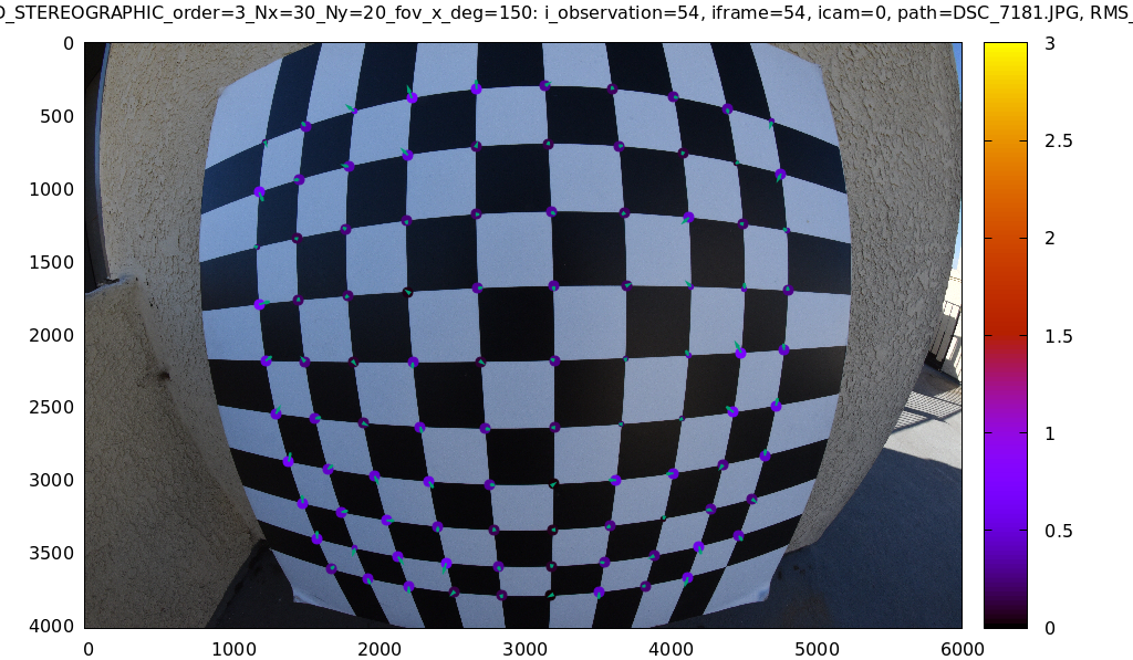
Let's look at the worst-fitting single image in this solve:
mrcal-show-residuals-board-observation \
  --from-worst                         \
  --vectorscale 100                    \
  --circlescale 0.5                    \
  --set 'cbrange [0:3]'                \
  splined.cameramodel                  \
  0

Interestingly, the worst observation here is the same one we saw with
LENSMODEL_OPENCV8. But all the errors are significantly smaller than before.
The previous radial pattern is much less pronounced, but it still there.
A sneak peek: this is caused by an assumption of a central projection (assuming that all rays intersect at a single point). An experimental and not-entirely-complete support for noncentral projection in mrcal exists, and works much better. The same frame, fitted with a noncentral projection:
This will be included in a future release of mrcal.
In any case, these errors are small, so let's proceed.
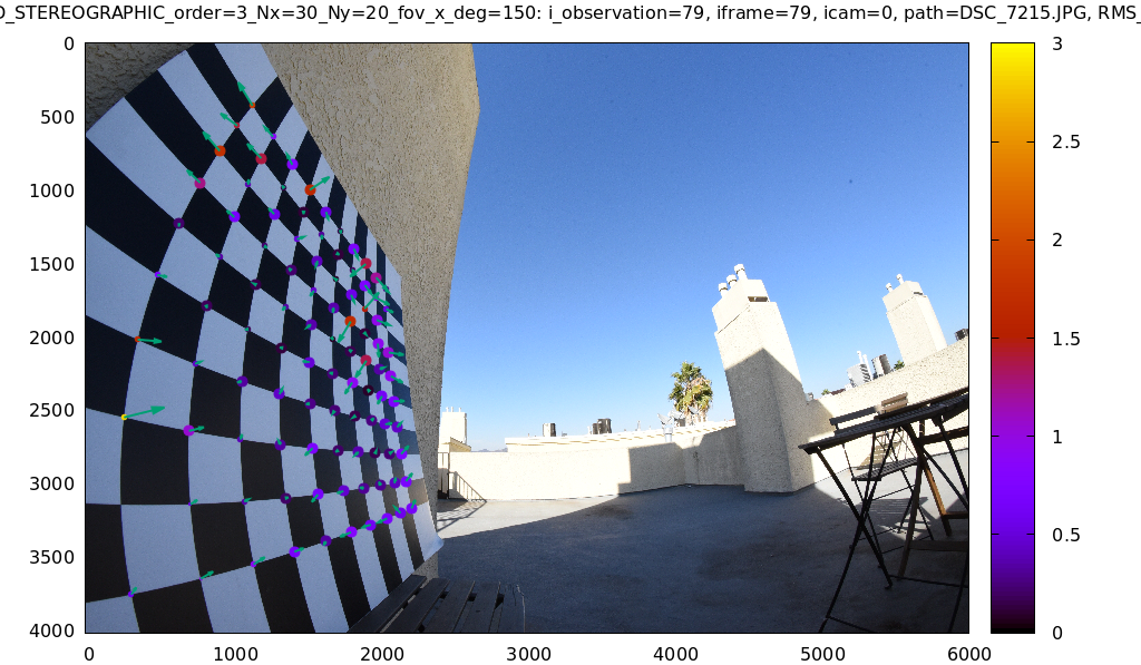
What happens when we look at the image that showed a poor fit in the corner previously? It was observation 79.
mrcal-show-residuals-board-observation \
  --vectorscale 100                    \
  --circlescale 0.5                    \
  --set 'cbrange [0:3]'                \
  splined.cameramodel                  \
  79
And the residual magnitudes of all the observations:
mrcal-show-residuals                   \
  --magnitudes                         \
  --set 'cbrange [0:3.5]'              \
  splined.cameramodel
Neat! The model fits the data in the corners now. And what about the residual directions?
mrcal-show-residuals    \
  --directions          \
  --unset key           \
  splined.cameramodel
Much better than before. Maybe there's still a pattern, but it's not clearly discernible.
We can also visualize the magnitude of the vector field defined by the splined surfaces \(\left| \Delta \vec u \right|\):
mrcal-show-splined-model-correction \
  --set 'cbrange [0:0.1]'           \
  --unset grid                      \
  splined.cameramodel
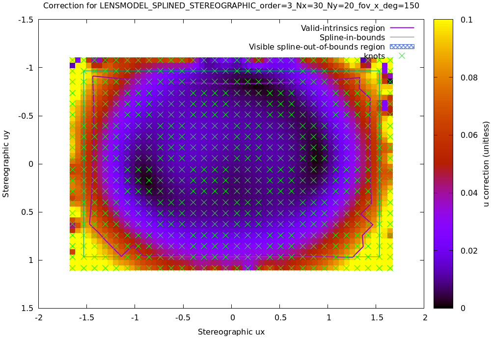
Each X in the plot is a "knot" of the spline surface, a point where a control point value is defined. We're looking at the spline domain, so the axes of the plot are the normalized stereographic projection coordinates \(u_x\) and \(u_y\), and the knots are arranged in a regular grid. The region where the spline surface is well-defined begins at the 2nd knot from the edges; its boundary is shown as a thin green line. The valid-intrinsics region (the area where the intrinsics are confident because we had sufficient chessboard observations there) is shown as a thick, purple curve. Since each \(\vec u\) projects to a pixel coordinate \(\vec q\) in some very nonlinear way, this curve is not straight.
We want the valid-intrinsics region to lie entirely within the spline-in-bounds region, and that happens here everywhere, except for a tiny sliver at the bottom-right. If some observations lie outside the spline-in-bounds regions, the projection behavior there will be less flexible than the rest of the model, resulting in less realistic uncertainties. See the lensmodel documentation for more detail.
Alternately, I can look at the spline surface as a function of the pixel coordinates. Just for \(\Delta u_x\):
mrcal-show-splined-model-correction \
  --set 'cbrange [0:0.1]'           \
  --imager-domain                   \
  --set 'xrange [-300:6300]'        \
  --set 'yrange [4300:-300]'        \
  --unset grid                      \
  splined.cameramodel
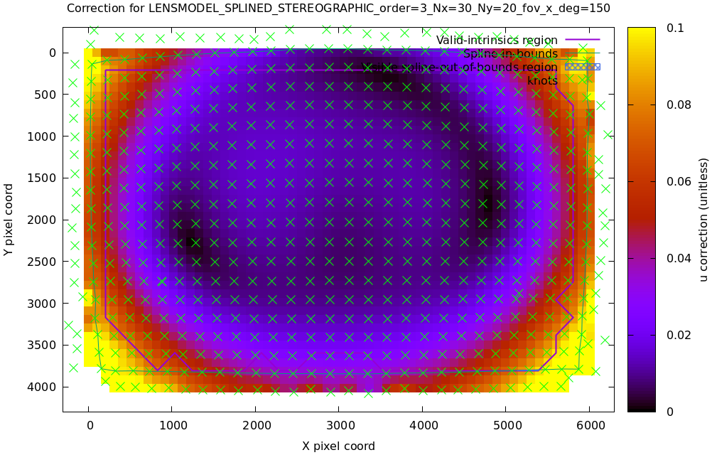
Now the valid-intrinsics region is a nice rectangle, but the spline-in-bounds region is complex curve. Projection at the edges is poorly-defined, so the boundary of the spline-in-bounds region appears irregular in this view.
I can also look at the correction vector field:
mrcal-show-splined-model-correction \
  --vectorfield \
  --imager-domain \
  --unset grid                      \
  --set 'xrange [-300:6300]'        \
  --set 'yrange [4300:-300]'        \
  --gridn 40 30 \
  splined.cameramodel

This doesn't show anything noteworthy in this solve, but seeing this is often informative with other lenses.