Model differencing
Table of Contents
Intrinsics differences
mrcal provides the mrcal-show-projection-diff tool to compute and display
projection differences between several models (implemented using
mrcal.show_projection_diff() and mrcal.projection_diff()). This has numerous
applications. For instance:
- evaluating the manufacturing variation of different lenses
- quantifying intrinsics drift due to mechanical or thermal stresses
- testing different solution methods
- underlying a cross-validation scheme
What is meant by a "difference"?
We want to compare different representations of the same lens, so we're not interested in extrinsics. At a very high level, to evaluate the projection difference at a pixel coordinate \(\vec q_0\) in camera 0 we need to:
- Unproject \(\vec q_0\) to a fixed point \(\vec p\) using lens 0
- Project \(\vec p\) back to pixel coords \(\vec q_1\) using lens 1
- Report the reprojection difference \(\vec q_1 - \vec q_0\)

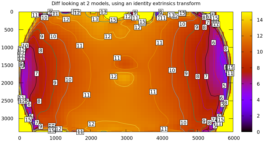
This simple definition is conceptually sound, but isn't applicable in practice. In the tour of mrcal we calibrated the same lens using the same data, but with two different lens models. The models are describing the same lens, so we would expect a low difference. However, the simple algorithm above produces a difference that is non-sensically high. As a heat map:
mrcal-show-projection-diff \
  --intrinsics-only        \
  --cbmax 15               \
  --unset key              \
  opencv8.cameramodel      \
  splined.cameramodel
And as a vector field:
mrcal-show-projection-diff \
  --intrinsics-only        \
  --vectorfield            \
  --vectorscale 5          \
  --gridn 30 20            \
  --cbmax 15               \
  --unset key              \
  opencv8.cameramodel      \
  splined.cameramodel

The reported differences are in pixels.
The issue is similar to the one encountered by the projection uncertainty routine: each calibration produces noisy estimates of all the intrinsics and all the coordinate transformations:

The above plots projected the same \(\vec p\) in the camera coordinate system, but that coordinate system shifts with each model computation. So in the fixed coordinate system attached to the camera housing, we weren't in fact projecting the same point.
There exists some transformation between the camera coordinate system from the solution and the coordinate system defined by the physical camera housing. It is important to note that this implied transformation is built-in to the intrinsics. Even if we're not explicitly optimizing the camera pose, this implied transformation is still something that exists and moves around in response to noise.
The above vector field suggests that we need to pitch one of the cameras. We can automate this by adding a critical missing step to the procedure above between steps 1 and 2:
- Transform \(\vec p\) from the coordinate system of one camera to the coordinate system of the other camera

We don't know anything about the physical coordinate system of either camera, so
we do the best we can: we compute a fit. The "right" transformation will
transform \(\vec p\) in such a way that the reported mismatches in \(\vec q\) will
be small. Previously we passed --intrinsics-only to bypass this fit. Let's
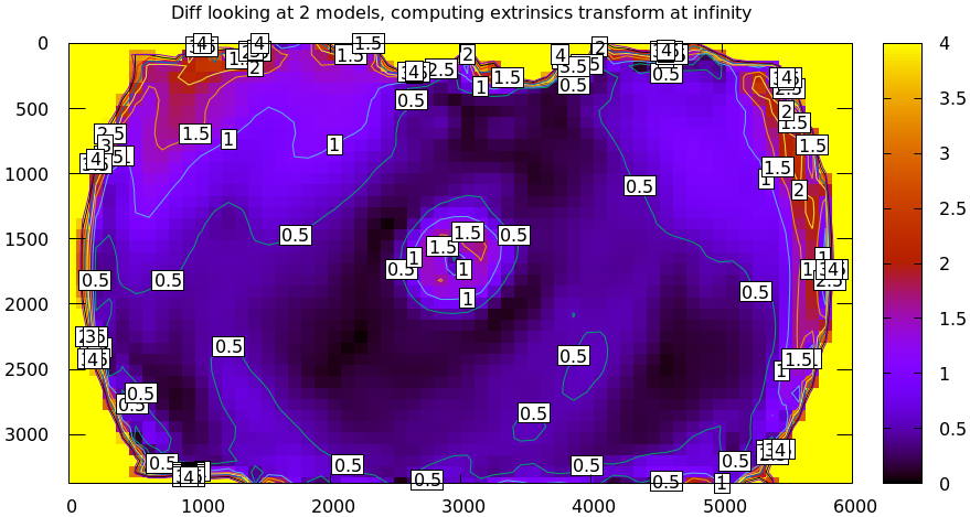
omit that option to get the the diff that we expect:
mrcal-show-projection-diff \
  --unset key              \
  opencv8.cameramodel      \
  splined.cameramodel
Implied transformation details
As with projection uncertainty, the difference computations are not invariant to range. So we always compute "the projection difference when looking out to \(r\) meters" for some possibly-infinite \(r\). The procedure we implement is:
- Regularly sample the two imagers, to get two corresponding sets of pixel coordinates \(\left\{\vec q_{0_i}\right\}\) and \(\left\{\vec q_{1_i}\right\}\)
- Unproject the camera-0 pixel coordinates to a set of points \(\left\{\vec
p_{0_i}\right\}\) in the camera-0 coordinate system. The range is given with
--distance.mrcal.sample_imager_unproject()function does this exactly - Unproject the camera-1 pixel coordiantes to a set of normalized unit observation vectors \(\left\{\vec v_{1_i}\right\}\) in the camera-1 coordinate system. These correspond to \(\left\{\vec p_{0_i}\right\}\), except they're unit vectors instead of points in space.
- Compute the implied transformation \(\left(R,t\right)\) as the one to maximize
\[ \sum_i w_i \vec v_{1_i}^T \frac{R \vec p_{0_i} + t}{\left|R \vec p_{0_i} +
t\right|} \] where \(\left\{w_i\right\}\) is a set of weights. As with main
calibration optimization, this one is unconstrained, using the
rttransformation representation. The inner product above is \(\cos \theta\) where \(\theta\) is the angle between the two observation vectors in the camera-1 coord system.
When looking out to infinity the \(t\) becomes insignificant, and we do a rotation-only optimization.
This is the logic behind mrcal.implied_Rt10__from_unprojections() and
mrcal.projection_diff().
Which transform is "right"?
We just described a differencing method that computes an implied transformation given a range \(r\). This will produce a different result for each \(r\), but in reality, there's only a single true transformation, and the solutions at different ranges are different estimates of it.
If we just need to compare two different representations of the same lens, then we don't care about the implied transformation itself. The correct thing to do here would be to set \(r\) to the intended working distance of the system: for me this is generally infinity. Looking at a single \(r\), these implied-transformation fits will always overfit a little bit, but from experience, this doesn't affect the resulting model-difference output.
However, in some applications (extrinsics differencing for instance), we do want the true implied transform. And when we look at this computed transform more deeply, we see that with some \(r\) we get a result that is clearly wrong. For instance:
$ mrcal-show-projection-diff \
    --no-uncertainties       \
    --unset key              \
    --distance 1000          \
    opencv8.cameramodel      \
    splined.cameramodel

Transformation cam1 <-- cam0:  rotation: 0.316 degrees, translation: [-2.67878241 -0.832383    1.8063095 ] m
## WARNING: fitted camera moved by 3.336m. This is probably aphysically high, and something is wrong. Pass both a high and a low --distance?
More on --no-uncertainties later; it's here to speed things up, and isn't
important. We asked for a diff at 1000m out, and the solver said that the
optimal transform moves the camera coordinate system back by 1.8m and to the
right by 2.7m. This is looking at the same data as before: comparing two solves
from the tour of mrcal. Nothing moved. The camera coordinate system could have
shifted inside the camera housing a tiny bit, but the solved shifts are huge,
and clearly aren't inside the housing anymore. This needs a deeper investigation
on how to do it "properly", but for practical use I have a working solution:
solve using points at two ranges at the same time, a near range and a far range:
$ mrcal-show-projection-diff \
    --no-uncertainties       \
    --unset key              \
    --distance 1,1000        \
    opencv8.cameramodel      \
    splined.cameramodel

Transformation cam1 <-- cam0:  rotation: 0.316 degrees, translation: [2.90213542e-05 2.59871714e-06 1.73397909e-03] m
Much better. This is analogous to the multiple ranges-to-the camera we need when we compute a surveyed calibration and the multiple ranges we get when we tilt the chessboard during calibration.
Selection of fitting data
When we use a fit to compute the implied transformation, we minimize the reprojection error. We hope that the main contributions to this error come from geometric misalignment. If this was the case, minimizing this reprojection error would produce the correct implied \(\left(R,t\right)\). Applying this transformation would correct the misalignment, leaving a very small residual. It is possible to have other error contributions though, which would break this method of finding the implied \(\left(R,t\right)\). This is common when intrinsics differences are significant; let's demonstrate that.
We just saw a difference result from the tour of mrcal, showing that the two models are similar but not identical. Once again:
mrcal-show-projection-diff \
  --unset key              \
  opencv8.cameramodel      \
  splined.cameramodel
This uses the default data-selection behavior of mrcal-show-projection-diff:
- uncertainties are used to weight the sampled points
- points are sampled from the whole imager (without uncertainties the default behavior is to use a limited region in the center instead)
What if we used all the data in the imager, but weighed them all equally?
mrcal-show-projection-diff \
  --unset key              \
  --no-uncertainties       \
  --radius 1e6             \
  --cbmax 50               \
  opencv8.cameramodel      \
  splined.cameramodel
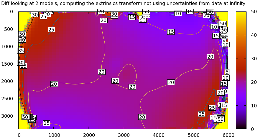
Note the completely different color-bar scaling: this difference is huge! The reason this doesn't work is that projections of the two models don't just differ due to an implied transformation: there's also a significant difference in intrinsics. This difference is small near the center, and huge in the corners, so even the optimal \(\left(R,t\right)\) fits badly. We can solve this problem by either
- Giving the bad points low weights during the solve by using the default
behavior, without
--no-uncertainties. This is described in the next section - Excluding the bad points entirely by passing a
--radius
Let's demonstrate the effect of --radius. I re-ran the calibration from the
tour of mrcal using LENSMODEL_OPENCV4. This model fits the wide lens even
worse than the LENSMODEL_OPENCV8 fits we studied, and is not expected to work
at all. But it is very good for this demo. If we run this solve, the outlier
rejection logic kicks in, and makes the solve converge despite the model not
fitting the data well. The resulting model is available here. Using an
insufficient model like this isn't a good way to run calibrations: the outlier
rejection will throw away the clearly-ill-fitting measurements, but marginal
measurements will make it through, which will slightly poison the result. I'm
only doing this for this demo. If you really do want to use an insufficient
model, and you really do care only about points near the center, you should use
the mrcal-cull-corners tool to throw away the data you don't care about, prior
to calibrating.
Let's compute the diff between the narrow-only LENSMODEL_OPENCV4 lens model
and the mostly-good-everywhere LENSMODEL_OPENCV8 model, using an expanding
radius of points. We expect this to work well when using a small radius, and we
expect the difference to degrade as we use more and more data away from the
center.
# This is a zsh loop
for r (200 600 800 1000) {
  mrcal-show-projection-diff \
    --no-uncertainties       \
    --distance 1             \
    --radius $r              \
    --cbmax 15               \
    --unset key              \
    --extratitle "radius $r" \
    opencv[48].cameramodel
}
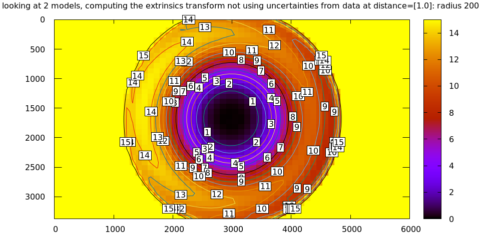
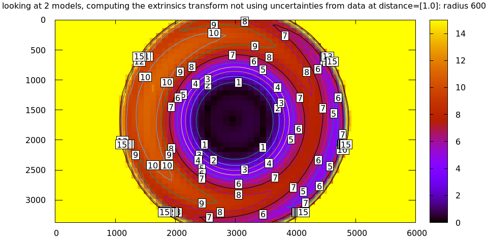
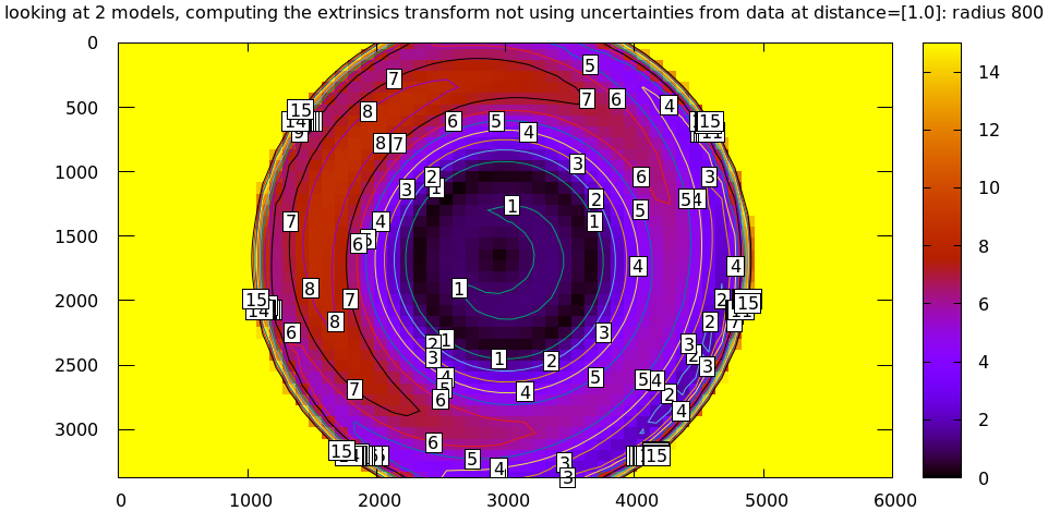
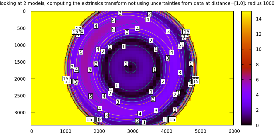
All of these radii are equally "right", and there's a trade-off in picking one. The models agree very well in a small region at the center, but they can also agree decently well in a much larger region, if we are willing to accept a higher level of error in the middle.
For the purposes of computing the implied transform you don't need a lot of
data, so I generally use a small region in the center, where I have reasonable
confidence that the intrinsics match. For a camera like this one --radius 500
is usually plenty.
Fit weighting
Clearly the LENSMODEL_OPENCV4 solve does agree with the LENSMODEL_OPENCV8
solve well, but only in the center of the imager. The issue from a tooling
standpoint is that in order for the tool to tell us that, we needed to tell
the tool to only look at the center. That is unideal.
The issue we observed is that some regions of the imager have unreliable behavior, which poisons the fit. But we know where the fit is reliable: in the areas where the projection uncertainty is low. So we can weigh the fit by the inverse of the projection uncertainty, and we will then favor the "good" regions. Without requiring the user to specify the good-projection region.
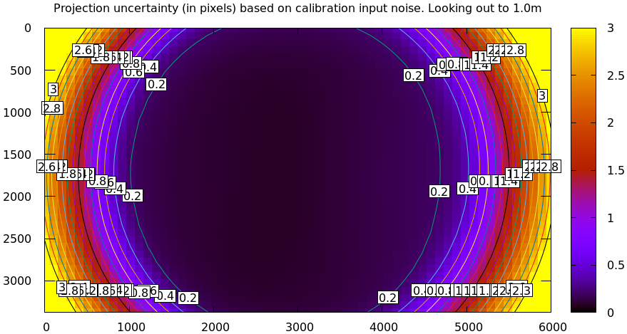
This works, but with a big caveat. As described on the projection uncertainty
page, lean models report overly-optimistic uncertainties. Thus when used as
weights for the fit, areas that actually are unreliable will be weighted too
highly, and will still poison the fit. We see that here, when comparing the
LENSMODEL_OPENCV4 and LENSMODEL_OPENCV8 results. The above plots show that
the LENSMODEL_OPENCV4 result is only reliable within a few 100s of pixels
around the center. However, LENSMODEL_OPENCV4 is a very lean model, so its
uncertainty at 1m out (near the sweet spot, where the chessboards were) looks
far better than that:
mrcal-show-projection-uncertainty \
    --distance 1                  \
    --unset key                   \
    opencv4.cameramodel
And the diff using that uncertainty as a weight without specifying a radius looks poor:
mrcal-show-projection-diff \
  --distance 1             \
  --unset key              \
  opencv[48].cameramodel

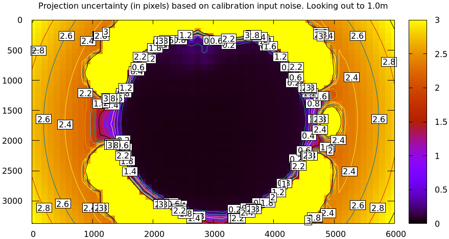
Where this technique does work well is when using splined models, which produce realistic uncertainty estimates. To demonstrate, let's produce a splined-model calibration that is only reliable in a particular region of the imager. We do this by culling the tour of mrcal calibration data to throw out all points outside of a circle at the center, calibrate off that data, and run a diff on those results:
< corners.vnl \
  mrcal-cull-corners --imagersize 6000 3376 --cull-rad-off-center 1500 \
> /tmp/raw.vnl &&
  vnl-join --vnl-sort - -j filename /tmp/raw.vnl \
     <(< /tmp/raw.vnl vnl-filter -p filename --has level |
                       vnl-uniq -c |
                       vnl-filter 'count > 20' -p filename ) \
  > corners-rad1500.vnl

mrcal-calibrate-cameras                                                         \
  --corners-cache corners-rad1500.vnl                                           \
  --lensmodel LENSMODEL_SPLINED_STEREOGRAPHIC_order=3_Nx=30_Ny=18_fov_x_deg=150 \
  --focal 1900                                                                  \
  --object-spacing 58.8e-3                                                      \
  --object-width-n 14                                                           \
  '*.JPG'

mrcal-show-projection-uncertainty \
  --distance 1                    \
  --unset key                     \
  splined-rad1500.cameramodel

mrcal-show-projection-diff \
  --distance 1             \
  --unset key              \
  splined{,-rad1500}.cameramodel
The cut-down corners are here and the resulting model is here. The uncertainty of this model looks like this:
and the diff like this:
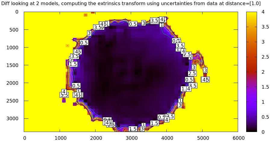
This is yet another reason to use only splined models for real-world lens modeling.
We just demonstrated that projection uncertainties provide a working method for
selecting the points used to fit the implied transformation. From a practical
standpoint, there's a downside: computing uncertainties makes the differencing
method much slower. So while the uncertainty-aware method is available in
mrcal-show-projection-diff, most of the time I run something like
mrcal-show-projection-diff --no-uncertainties --radius 500. This falls back on
simply using the points in a 500-pixel-radius circle at the center. This
computes much faster, and with good-coverage-low-error calibrations usually
produces a very similar result. If something looks odd, I will run the
uncertainty-aware diff to debug. But my usual default is --no-uncertainties.
Extrinsics differences
The above technique can be used to quantify intrinsics differences between two representations of the same lens. This is useful, for instance, to detect any intrinsics calibration drift over time. This doesn't tell us anything about extrinsics drift, however. It's possible to have a multi-camera system composed of very stable lenses mounted on a not-rigid-enough mount. Any mechanical stress wouldn't affect the intrinsics, but the extrinsics would shift. And we want a method to quantify this shift .
I haven't needed to do this very often, so the technique I'm using isn't mature
yet. The extrinsics diff computation is implemented in the
extrinsics-stability.py tool. This isn't stable yet, and only exists in the
mrcal sources for now. But I used it several times, and it appears to work well.
In this description I will consider 2-camera systems, but the approach is general for any number of cameras. Let's say we have two calibrations (0 and 1) of a stereo pair (\(\mathrm{left}\) and \(\mathrm{right}\) cameras). Between the calibrations the system was stressed (shaked, flipped, heated, etc), and we want to know if the camera geometry shifted as a result. The obvious technique is to compare the transformation \(T_{0\mathrm{left},0\mathrm{right}}\) and \(T_{1\mathrm{left},1\mathrm{right}}\). Each of these is available directly in the two calibrations, and we can compute the difference \(T_{0\mathrm{right},1\mathrm{right}} = T_{0\mathrm{right},0\mathrm{left}} T_{1\mathrm{left},1\mathrm{right}}\). This is the transform between the right cameras in the two calibrations if we line up the two left cameras.
This approach sounds good, but it is incomplete because it ignores the transformation implied by the different intrinsics, as described above. So lining up the two left cameras does not line up their projection behavior. And comparing the poses of the right cameras does not compare their projection behavior.
We just talked about how to compute the implied transforms \({T^\mathrm{implied}_{0\mathrm{left},1\mathrm{left}}}\) and \(T^\mathrm{implied}_{0\mathrm{right},1\mathrm{right}}\). So the final transformation describing the shift of the right camera is
\[ T^\mathrm{implied}_{1\mathrm{right},0\mathrm{right}} T_{0\mathrm{right},0\mathrm{left}} T^\mathrm{implied}_{0\mathrm{left},1\mathrm{left}} T_{1\mathrm{left},1\mathrm{right}} \]
The extrinsics-stability.py tool implements this logic. To compute the implied
transformations we want the "true" transform, not a transform at any particular
range, so we use a near and a far range.
I tried this out in practice on a physical camera pair. I had calibrations before and after a lot of mechanical jostling happened. And for each calibration I had an odd and even set for cross-validation, which reported very low intrinsics differences: the intrinsics were "correct". I evaluated the extrinsics stability, looking at the odd calibrations:
$ ~/projects/mrcal/analyses/extrinsics-stability.py \
  BEFORE/camera-0-odd-SPLINED.cameramodel           \
  BEFORE/camera-1-odd-SPLINED.cameramodel           \
  AFTER/camera-0-odd-SPLINED.cameramodel            \
  AFTER/camera-1-odd-SPLINED.cameramodel

translation: 0.04mm in the direction [0.13 0.06 0.99]
rotation:    0.01deg around the axis [ 0.93  0.32 -0.18]
So it claims that the right camera shifted by 0.04mm and yawed by 0.01deg. This sounds low-enough to be noise, but what is the noise level? The tool also reports the camera resolution for comparison against the reported rotation:
Camera 0 has a resolution of 0.056 degrees per pixel at the center
Camera 1 has a resolution of 0.057 degrees per pixel at the center
Camera 2 has a resolution of 0.056 degrees per pixel at the center
Camera 3 has a resolution of 0.057 degrees per pixel at the center
So this rotation is far smaller than one pixel. What if we look at the allegedly-identical "even" calibration:
$ ~/projects/mrcal/analyses/extrinsics-stability.py \
  BEFORE/camera-0-even-SPLINED.cameramodel          \
  BEFORE/camera-1-even-SPLINED.cameramodel          \
  AFTER/camera-0-even-SPLINED.cameramodel           \
  AFTER/camera-1-even-SPLINED.cameramodel

translation: 0.07mm in the direction [ 0.63 -0.73  0.25]
rotation:    0.00deg around the axis [ 0.55 -0.32  0.77]
That's similarly close to 0. What if instead of comparing before/after we compare odd/even before and then odd/even after? odd/even happened at the same time, so there was no actual shift, and the result will be at the noise floor.
$ ~/projects/mrcal/analyses/extrinsics-stability.py \
  BEFORE/camera-0-odd-SPLINED.cameramodel           \
  BEFORE/camera-1-odd-SPLINED.cameramodel           \
  BEFORE/camera-0-even-SPLINED.cameramodel          \
  BEFORE/camera-1-even-SPLINED.cameramodel

translation: 0.07mm in the direction [0.09 0.76 0.64]
rotation:    0.00deg around the axis [ 0.77 -0.1  -0.63]


$ ~/projects/mrcal/analyses/extrinsics-stability.py \
  AFTER/camera-0-odd-SPLINED.cameramodel            \
  AFTER/camera-1-odd-SPLINED.cameramodel            \
  AFTER/camera-0-even-SPLINED.cameramodel           \
  AFTER/camera-1-even-SPLINED.cameramodel

translation: 0.05mm in the direction [9.69e-01 8.13e-04 2.46e-01]
rotation:    0.00deg around the axis [-0.43 -0.78  0.44]
So with these calibrations we have strong evidence that no extrinsics drift has occurred. More testing and development of this method are planned, and this tool will be further documented and released.