How to run a calibration
Table of Contents
Calibrating cameras is one of the main applications of mrcal, so I describe this process in some detail here.
Capturing images
Calibration object
We need to get images of a calibration object, a board containing an observable grid of points. mrcal doesn't care where these observations come from: any tool that can produce a table of corner observations can be utilized. Currently the recommended method is to use a classical chessboard target, and to employ the mrgingham detector. The mrgingham documentation has a .pdf of a chessboard pattern that works well. See the recipes to use a non-mrgingham detector and/or a non-chessboard object.
Chessboard shape
The pattern should be printed and mounted onto a rigid and flat surface to produce the calibration object. The optimization problem assumes the board shape to be constant over all the calibration images, and any instability in the board shape breaks that assumption. Depending on the resolution of the camera and the amount of calibration accuracy required, even a slightly floppy chessboard can break things. Don't take this for granted. A method for quantifying this effect appears below.
Similarly, the optimization problem assumes that the calibration object is mostly flat. Some amount of deformation is inevitable, so mrcal does support a simple non-planar board model, with the board shape being computed as part of the calibration solve. In my experience, if you try to make sure the board is flat, this model is enough to fix most of the unavoidable small deflections. If care isn't taken to ensure the board is flat, the current simple deformation model is often insufficient to fully model the shape. Don't take this for granted either. A method for quantifying this effect appears below as well.
I usually use a square chessboard roughly 1m per side to calibrate my fisheye lenses. Such a large chessboard often has issues with its shape. To mitigate these, my chessboard is backed by about 1 inch of aluminum honeycomb. This is expensive, but works well to stabilize the shape. The previous board I was using is backed with the same amount of foam instead. This is significantly cheaper, and still pretty good, but noticeably less flat and less rigid. This foam-backed board does warp with variations in temperature and humidity, but this drift is slow, and the shape is usually stable long-enough for a chessboard dance. If you can make one, the aluminum honeycomb-backed boards are strongly recommended.
Chessboard size
There's a tradeoff to consider between large and small chessboards. According to the dance study, we want close-ups that fill the imager, so we're choosing between small chessboards placed near the camera and large chessboards placed away from the camera.
- Small chessboards placed close to the camera produce two issues:
- the chessboard would appear out of focus. This is OK up to a point (out-of-focus blur is mostly isotropic, and this noise averages out nicely), but extreme out-of-focus images should probably be avoided
- Extreme close-ups exhibit noncentral projection behavior: observation rays don't all intersect at the same point. Today's mrcal cannot model this behavior, so extreme close-ups should be avoided to allow the central-only models to fit. The cross-validation page shows how to detect errors caused by noncentral projection
- Large chessboards are better, but are difficult to manufacture, to keep them flat and stiff, and to move them around. Currently I use a 1m x 1m square board, which seems to be near the limit of what is reasonable.
For wide lenses especially, you want a larger chessboard. When calibrating an unfamiliar system I usually try running a calibration with whatever chessboard I already have, and then analyze the results to see if anything needs to be changed. It's also useful to rerun the dance study for the specific geometry being calibrated.
Image-capturing details
Now that we have a calibration object, this object needs to be shown to the camera(s). It is important that the images contain clear features. Motion blur or exposure issues will all cause bias in the resulting calibration.
If calibrating multiple cameras, mrcal will solve for all the intrinsics and extrinsics. There is one strong requirement on the captured images in this case: the images must be synchronized across all the cameras. This allows mrcal to assume that if camera A and camera B observed a chessboard at time T, then this chessboard was at exactly the same location when the two cameras saw it. Generally this means that either
- The cameras are wired to respond to a physical trigger signal
- The chessboard and cameras were physically fixed (on a tripod, say) at each time of capture
Some capture systems have a "software" trigger mode, but this is usually too loose to produce usable results. A similar consideration exists when using cameras with a rolling shutter. With such cameras it is imperative that everything remain stationary during image capture, even when only one camera is involved. See the residual analysis of synchronization errors and of rolling shutter for details.
Lens settings
Lens intrinsics are usually very sensitive to any mechanical manipulation of the lens. It is thus strongly recommended to set up the lens it its final working configuration (focal length, focus distance, aperture), then to mechanically lock down the settings, and then to gather the calibration data. This often creates dancing challenges, described in the next section.
If you really need to change the lens settings after calibrating or if you're concerned about drifting lens mechanics influencing the calibration (you should be!), see the recipes for a discussion.
Dancing
As shown in the dance study, the most useful observations to gather are
- close-ups: the chessboard should fill the whole frame as much as possible.
- oblique views: tilt the board forward/back and left/right. I generally tilt by ~ 45 degrees. At a certain point the corners become indistinct and the detector starts having trouble, but depending on the lens, that point could come with quite a bit of tilt. A less dense chessboard eases this also, at the cost of requiring more board observations to get the same number of points.
- If calibrating multiple cameras, it is impossible to place a calibration object at a location where it's seen by all the cameras and where it's a close-up for all the cameras. So you should get close-ups for each camera individually, and also get observations common to multiple cameras, that aren't necessarily close-ups. The former will serve to define your camera intrinsics, and the latter will serve to define your extrinsics (geometry). Get just far-enough out to create the joint views. If usable joint views are missing, the extrinsics will be undefined, and the solver will complain about a "not positive definite" (singular in this case) Hessian.
A dataset composed primarily of tilted closeups produces good results.
As described above, you want a large chessboard placed as close to the camera as possible, before the out-of-focus and noncentral effects kick in.
If the model will be used to look at far-away objects, care must be taken to produce a reliable calibration at long ranges, not just at the short ranges where the chessboards were. The primary way to do that is to get close-up chessboard views. If the close-up range is very different from the working range (infinity, possibly), the close-up images could be very out-of-focus. The current thought is that the best thing to do is to get close-up images even if they're out of focus. The blurry images will have a high uncertainty in the corner observations (hopefully without bias), but the uncertainty improvement that comes from the near-range chessboard observations more than makes up for it. In these cases you usually need to get more observations than you normally would to bring down the uncertainties to an acceptable level. In challenging situations it's useful to re-run the dance study for the specific use case to get a sense of what kind of observations are required and what kind of uncertainties can be expected. See the dance study for detail.
Another issue that could be caused by extreme close-ups is a noncentral projection behavior: observation rays don't all intersect at the same point. Today's mrcal cannot model this behavior, and the cross-validation would show higher-than-expected errors. In this case it is recommended to gather calibration data from further out.
It is better to have more chessboard data rather than less. mrgingham will throw away frames where no chessboard can be found, so it is perfectly reasonable to grab too many images with the expectation that they won't all end up being used in the computation. I usually aim for about 100 usable frames, but you may get away with fewer, depending on your specific scenario. The mrcal uncertainty feedback will tell you if you need more data.
Naturally, intrinsics are accurate only in areas where chessboards were observed: chessboard observations on the left side of the image tell us little about lens behavior on the right side. Thus it is imperative to cover the whole field of view during the chessboard dance. It is often tricky to get good data at the edges and corners of the imager, so care must be taken. Some chessboard detectors (mrgingham in particular) only report complete chessboards. This makes it extra-challenging to obtain good data at the edges: a small motion that pushes one chessboard corner barely out of bounds causes the whole observation to be discarded. It is thus very helpful to be able to see a live feed of the camera as the images are being captured. In either case, checking the coverage is a great thing to do. The usual way to do this is indirectly: by visualizing the projection uncertainty. Or by visualizing the obtained chessboard detections directly.
Image file-naming convention
With monocular calibrations, there're no requirements on image filenames: use
whatever you like. If calibrating multiple synchronized cameras, however, the
image filenames need to indicate which camera captured each image and at which
time. I generally use frameFFF-cameraCCC.jpg. Images with the same FFF are
assumed to have been captured at the same instant in time, and CCC identifies
the camera. Naming images in this way is sufficient to communicate these
mappings to mrcal.
Detecting corners
A number of tools are available to detect chessboard corners (OpenCV is commonly
used, and different organizations have their own in-house versions). None of the
available ones worked well for my use cases, so I had to write my own, and I
recommend it for all corner detections: mrgingham. mrgingham is fast and is
able to find chessboard corners subject to very un-pinhole-like projections. At
this time it has two limitations that will be lifted eventually:
- It more or less assumes a regular grid of N-by-N corners (i.e. N+1-by-N+1 squares)
- It requires all the corners to be observed in order to report the detections from an image. Incomplete chessboard observations aren't supported
If these are unacceptable, any other detector may be used instead. See the recipes.
Using mrgingham
Once mrgingham is installed or built from source, it can be run by calling the
mrgingham executable. The sample in the tour of mrcal processes these images
to produce these chessboard corners like this:
mrgingham --jobs 4 --gridn 14 '*.JPG' > corners.vnl
mrgingham tries to handle a variety of lighting conditions, including varying illumination across the image, but the corners must exist in the image in some form.
At this time mrgingham returns only complete chessboard views: if even one corner of the chessboard couldn't be found, mrgingham will discard the entire image. Thus it takes care to get data at the edges and in the corners of the imager. A live preview of the captured images is essential.
Another requirement due to the design of mrgingham is that the board should be held with a flat edge parallel to the camera xz plane (parallel to the ground, usually). mrgingham looks for vertical and horizontal sequences of corners, but if the board is rotated diagonally, then none of these sequences are clearly "horizontal" or "vertical".
Choice of calibration object
When given an image of a chessboard, the detector is directly observing the feature we actually care about: the corner. Another common calibration board style is a grid of circles, where the feature of interest is the center of each circle. When given an image of such a grid of circles, the detector either
- detects the contour at the edge of each circle
- finds the pixel blob comprising each circle observation
and from either of these, the detector infers the circle center. This can work when looking at head-on images, but when given tilted images subjected to non-pinhole lens behaviors, getting accurate circle centers from outer contours or blobs is hard. The resulting inaccuracies in the detections of circle centers will introduce biases into the solve that aren't modeled by the projection uncertainty routine, so chessboards are strongly recommended in favor of circle grids.
Some other calibration objects use AprilTags. mrcal assumes independent noise on each point observation, so correlated sources of point observations are also not appropriate sources of data. Thus using individual corners of AprilTags will be un-ideal: their noise is correlated. Using the center of an AprilTag would eliminate this correlated noise, but maybe would have a similar inaccuracy problem that a grid of circles would have.
If using a possibly-problematic calibration object such as a grid of circles or AprilTags, double-check the detections by reprojecting to calibration-object space after a solve has completed.
Visualization
Once we have a corners.vnl from some chessboard detector, we can visualize the
coverage. From the tour of mrcal:
$ < corners.vnl       \
  vnl-filter -p x,y | \
  feedgnuplot --domain --square --set 'xrange [0:6000] noextend' --set 'yrange [3376:0] noextend'
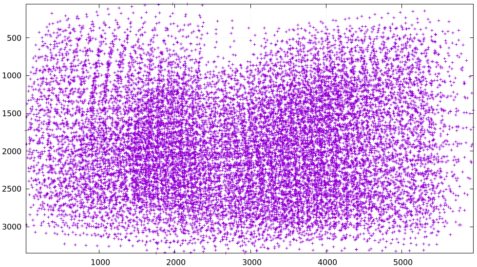
Doing this is usually unnecessary since the projection uncertainty reporting shows the coverage (and more!), but it's good to be able to do this for debugging.
Model choice
Before calibrating we need to choose the model for representing the lenses. Use
LENSMODEL_SPLINED_STEREOGRAPHIC. This model works very well, and is able to
represent real-world lenses better than the parametric models (all the other
ones). This is true even for long, near-pinhole lenses. Depending on the
specific lens and the camera resolution this accuracy improvement may not be
noteworthy. But even in those cases, the splined model is flexible enough to get
truthful projection uncertainty estimates, so it's still worth using. Today I
use other models only if I'm running quick experiments: splined models have many
more parameters, so things are slower.
LENSMODEL_SPLINED_STEREOGRAPHIC has several configuration variables that need
to be set. The full implications of these choices still need to be studied, but
the results appear fairly insensitive to these. I generally choose order=3 to
select cubic splines. I generally choose a rich model with fairly dense spline
spacing. For instance the splined model used in the tour of mrcal has
Nx=30_Ny=18. This has 30 spline knots horizontally and 18 vertically. You
generally want Ny / Nx to roughly match the aspect ratio of the imager. The
Nx=30_Ny=18 arrangement is probably denser than it needs to be, but it works
OK. The cost of such a dense spline is a bit of extra computation time and more
stringent requirements on calibration data to fully and densely cover the
imager.
The last configuration parameter is fov_x_deg: the horizontal field-of-view of
the lens. The splined model is defined by knots spread out across space, the
arrangement of these knots defined by the fov_x_deg parameter. We want the
region in space defined by the knots to roughly match the region visible to the
lens. A too-large fov_x_deg would waste some knots by placing them beyond
where the lens can see. And a too-small fov_x_deg would restrict the
projection representation on the edge of the image.
An initial estimate of fov_x_deg can be computed from the datasheet of the lens.
Then a test calibration should be computed using that value, and the
mrcal-show-splined-model-correction tool can then be used to validate that
fov_x_deg parameter. In the tour of mrcal we get something like this:
mrcal-show-splined-model-correction   \
  --set 'cbrange [0:0.1]'             \
  --unset grid                        \
  --set 'xrange [:] noextend'         \
  --set 'yrange [:] noextend reverse' \
  --set 'key opaque box'              \
  splined.cameramodel
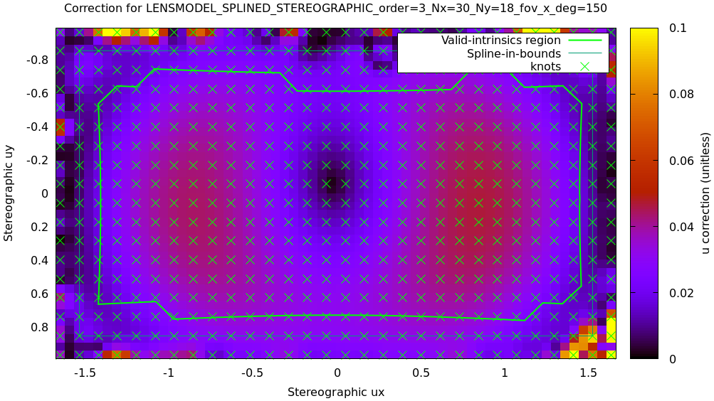
This is about what we want. The valid-intrinsics region covers most of the spline-in-bounds region without going out-of-bounds anywhere. In the tour of mrcal we followed this procedure to end up with
LENSMODEL_SPLINED_STEREOGRAPHIC_order=3_Nx=30_Ny=18_fov_x_deg=150
Getting this perfect isn't important, so don't spent a ton of time working on it. See the lensmodel documentation for more detail.
Computing the calibration
We have data; we have a lens model; we're ready. Let's compute the calibration
using the mrcal-calibrate-cameras tool. The invocation should look something
like this:
mrcal-calibrate-cameras                                                         \
  --corners-cache corners.vnl                                                   \
  --lensmodel LENSMODEL_SPLINED_STEREOGRAPHIC_order=3_Nx=30_Ny=18_fov_x_deg=150 \
  --focal 1900                                                                  \
  --object-spacing 0.0588                                                       \
  --object-width-n 14                                                           \
  '*.JPG'
--corners-cache corners.vnlsays that the chessboard corner coordinates live in a file calledcorners.vnl. This is the output of the corner detector. If this argument is omitted, or a non-existent file is given,mrcal-calibrate-cameraswill run mrgingham, and write the results into the given path. Thus the same command would be used to both compute the corners initially, and to reuse the pre-computed corners in subsequent runs.As described above, the
corners.vnlfile can come from any chessboard detector. If it's a detector that produces a 4th column of weights instead of a decimation level, pass in--corners-cache-has-weights--lensmodelspecifies which lens model we're using for all the cameras. See the "Model choice" section above. Not being able to select different models for different cameras is a current limitation of mrcal. If some very different lenses are present in the same calibration, I use a densely-spaced (highNx,Ny) splined model with thefov_x_degof the widest lens in the set. This wastes knots in the too-wide areas of the narrow lenses, but if the spline was dense-enough, there're enough knots remaining to fit the narrower lenses.--focal 1900provides the initial estimate for the camera focal lengths, in pixels. This doesn't need to be extremely precise, but do try to get this close if possible. The focal length value to pass to--focal(\(f_\mathrm{pixels}\)) can be derived using the stereographic model definition:
\[ f_\mathrm{pixels} \approx \frac{\mathrm{imager\_width\_pixels}}{4 \tan \frac{\mathrm{field\_of\_view\_horizontal}}{4}} \]
This expression is a good initial estimate for both long and wide lenses. Note that the manufacturer-specified "field of view" and "focal length" values are usually poorly-defined: the former is different in all directions, and the latter is meaningless in wide lenses that are nowhere near the pinhole model. With a longer lens, we can assume pinhole behavior to get
\[ f_\mathrm{pixels} = f_\mathrm{mm} \frac{\mathrm{imager\_width\_pixels}}{\mathrm{imager\_width\_mm}} \]
As with the fov_x_deg parameter described in the "Model
choice" section above, running a test calibration with a rough estimate, and
then passing in the much-closer optimized value is a good strategy. The
optimized focal length is the first two values of the intrinsics vector in
the result. Those two values should be similar, and anything around there
should work well for --focal.
--object-spacingis the distance between neighboring corners in the chessboard. Even spacing, identical in both directions is assumed--object-width-nis the horizontal corner count of the calibration object. In the example invocation above there is no--object-height-n, somrcal-calibrate-camerasassumes a square chessboard
After the options, mrcal-calibrate-cameras takes globs describing the images.
One glob per camera is expected, and in the above example one glob was given:
'*.JPG'. Thus this is a monocular solve. More cameras would imply more globs.
For instance a 2-camera calibration might take arguments
'frame*-camera0.png' 'frame*-camera1.png'
Note that these are globs, not filenames. So they need to be quoted or
escaped to prevent the shell from expanding them: hence '*.JPG' and not
*.JPG.
Finally, to compute cross-validation diffs (see below) it's necessary to run
several independent calibrations. I generally split the dataset into even/odd
chunks, and calibrate them independently. With this zsh snippet, for instance:
for oddeven (odd even) {

    cmd=(mrcal-calibrate-cameras                                                       \
         --corners-cache corners.vnl                                                   \
         --lensmodel LENSMODEL_SPLINED_STEREOGRAPHIC_order=3_Nx=30_Ny=18_fov_x_deg=150 \
         --focal 1900                                                                  \
         --object-spacing 0.0588                                                       \
         --object-width-n 14)

    if [[ $oddeven = "even" ]] {
        globs=('frame*[02468]-camera'{0,1}'.png')
    } else {
        globs=('frame*[13579]-camera'{0,1}'.png')
    }

    cmd=($cmd $globs)

    $cmd

    for i (0 1) {
        mv camera-$i.cameramodel camera-$i-$oddeven.cameramodel
    }
}
Troubleshooting broken solves
Usually the solver converges, and produces a result. Then we look at the diagnostics to evaluate the quality of this result (next section). We can do that if the errors are small, and the optimization completed successfully. If the data issues are too large, however (pervasive sync errors, completely insufficient lens model, etc), the solver will have trouble. It could
- Take a very long time to converge to some solution
Produce tool many outliers, possibly incrementally, producing output such as this:
mrcal.c(5413): Threw out some outliers. New count = 174/35280 (0.5%). Going again
mrcal.c(5413): Threw out some outliers. New count = 252/35280 (0.7%). Going again
mrcal.c(5413): Threw out some outliers. New count = 303/35280 (0.9%). Going again
This will slow down the solve dramatically. Unless the data is known to be funky, more than ~ 3% outliers should raise questions
If the solver has trouble like this, it is usually helpful to turn off the
outlier rejection by running mrcal-calibrate-cameras --skip-outlier-rejection
...., and then examine the residuals as described below. Hopefully that would
provide a hint about the issues.
It also helps to simplify the problem, which is effective at isolating certain issues. For instance, a nonconverging multi-camera solve should be attempted monocularly, one camera at a time. If some cameras converge and some don't, that points to the issue. If individually the solves converge, but together they don't, there could be an issue with the camera synchronization, or the chessboard corner indices aren't consistent. Similarly solving with a subset of images is often enlightening.
Another common problem is getting messages like this:
mrcal.c(3758): WARNING: Board observation 157 (icam_intrinsics=0, icam_extrinsics=-1, iframe=104) had almost all of its points thrown out as outliers: only 0/100 remain. CHOLMOD is about to complain about a non-positive-definite JtJ. Something is wrong with this observation
mrcal.c(3758): WARNING: Board observation 158 (icam_intrinsics=1, icam_extrinsics=0, iframe=104) had almost all of its points thrown out as outliers: only 0/100 remain. CHOLMOD is about to complain about a non-positive-definite JtJ. Something is wrong with this observation
mrcal.c(5412): Threw out some outliers (have a total of 861 now); going again
libdogleg at dogleg.c:1115: CHOLMOD warning:
libdogleg at dogleg.c:1115:  not positive definite.
libdogleg at dogleg.c:1115:  file: ../Cholesky/t_cholmod_rowfac.c
libdogleg at dogleg.c:1115:  line: 430
libdogleg at dogleg.c:1115:
The complaint is about a singular Hessian matrix. Usually this happens if some variable in the optimization has no effect at all on the solution, and the optimizer thus doesn't know what to do with that variable. Usually heavy outlier rejection precedes this, and the missing data is causing the problem. Example: all chessboard observations for a given frame were thrown out; thus moving the chessboard pose at that time has no effect, and we get a singular Hessian. The diagnostic technique is the same: disable the outlier rejection and examine the residuals.
Interpreting the results
Once we have a calibration, we should evaluate how well it represents reality.
The tour of mrcal shows a very detailed process: a real-world fit using
LENSMODEL_OPENCV8 and a real-world fit using
LENSMODEL_SPLINED_STEREOGRAPHIC_.... The analysis sequence outlined there is
too thorough for everyday use, but it's good to look through those pages to get
a sense. A high-level process is
- Examine the projection uncertainty to make sure we have enough good data in the right places
- Examine the cross-validation diffs to confirm that the model fits and that the reported uncertainty is trustworthy
- If these diffs are too high, examine the residuals to find out why
This is a lot, but you don't need to do all this every time. As noted in the noise model description, we want homoscedastic noise in our observations of the chessboard corners. We will get that if and only if our models faithfully describe the world; so the available diagnostics serve to pinpoint areas where the models don't fit, so that those issues could be addressed.
I now describe each step.
Projection uncertainty
Today I'm primarily concerned with the uncertainty in the intrinsics. As described in detail in the projection-uncertainty page, the projection uncertainty computed by mrcal gauges the effect of sampling error. Since we always have noise in our chessboard observations, it's important that the solution be insensitive to this noise. Otherwise a recalibration of the same system would produce very different results due to new chessboard observations containing new noise.
Projection uncertainty can be visualized with the
mrcal-show-projection-uncertainty tool. From the tour of mrcal:
mrcal-show-projection-uncertainty splined.cameramodel --cbmax 1 --unset key
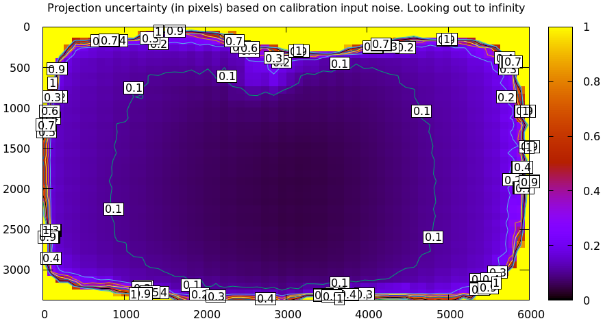
This is projection uncertainty at infinity, which is what I'm usually interested
in. If we care only about the performance at some particular distance, that
can be requested with mrcal-show-projection-uncertainty --distance .... That
uncertainty will usually be better than the uncertainty at infinity. Making sure
things work at infinity will make things work at other ranges also.
The projection uncertainty measures the quality of the chessboard dance. If the guidelines noted above were followed, you'll get good uncertainties. If the uncertainty is poor in some region, you need more chessboard observations in that area. To improve it everywhere, follow the guidelines: more observations, more closeups, more tilt.
The projection uncertainties will be overly-optimistic if model errors are present or if a too-lean lens model is selected. So we now look at the cross-validation diffs to confirm that no model errors are present. If we can confirm that, the projection uncertainties can be used as the authoritative gauge of the quality of our calibration.
Since the uncertainties are largely a function of the chessboard dance, I usually don't bother looking at them if I'm recalibrating a system that I have calibrated before, with a similar dance. Since the system and the dance didn't change, neither would the uncertainty.
Cross-validation diffs
If we have an acceptable projection uncertainty, we need to decide if it's a good gauge of calibration quality: if we have model errors or not.
A good way to do that is to compute a cross-validation: we calibrate the camera system twice with independent input data, and we compare the resulting projections. If the models fit, then we only have sampling error affecting the solves, and the resulting differences will be in-line with what the uncertainties predict: \(\mathrm{difference} \approx \mathrm{uncertainty}_0 + \mathrm{uncertainty}_1\). Otherwise, we have an extra source of error not present in the uncertainty estimates, which would cause the cross-validation diffs to be significantly higher. That would suggest a deeper look is necessary. See the tour of mrcal for more about the connection between uncertainty and cross-validation.
To get the data, we can do two separate dances, or we can split the dataset into odd/even images, as described above. Note: if the chessboard is moved very slowly, the even and odd datasets will be very qualitatively similar, and it's possible to get a low cross-validation diff even in the presence of model errors: the two samples of the model error distribution would be similar to each other. This usually doesn't happen, but keep in mind that it could, so you should move at a reasonable speed to make the odd/even datasets non-identical.
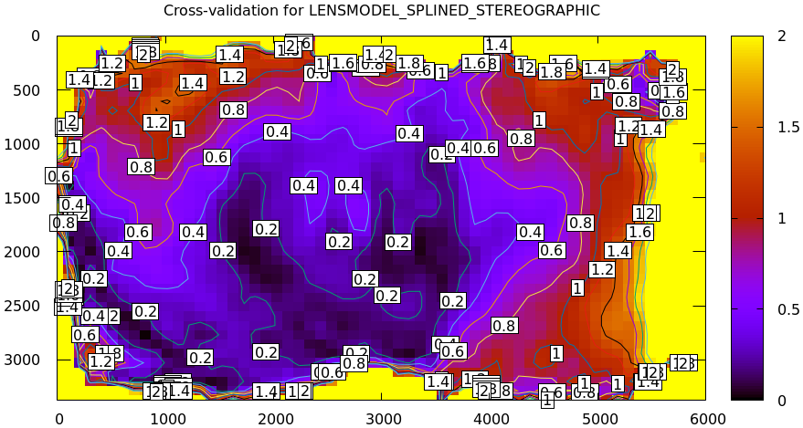
In the tour of mrcal we computed a cross-validation, and discovered that there indeed exists a model error. The cross-validation diff looked like this:
mrcal-show-projection-diff           \
  --cbmax 2                          \
  --unset key                        \
  2-f22-infinity.splined.cameramodel \
  3-f22-infinity.splined.cameramodel
And the two uncertainties looked roughly like this:
The diff is more than roughly 2x the uncertainty, so something wasn't fitting: the lens had a non-negligible noncentral behavior at the chessboard distance, which wasn't fixable with today's mrcal. So we could either
- Accept the results as is, using the diffs as a guideline to how trustworthy the solves are
- Gather more calibration images from further out, minimizing the unmodeled noncentral effect
Cross-validation diffs are usually very effective at detecting issues, and I usually compute these every time I calibrate a lens. In my experience, these are the single most important diagnostic output.
While these are very good at detecting issues, they're less good at pinpointing the root cause. To do that usually requires thinking about the solve residuals (next section).
Residuals
We usually have a lot of images and a lot of residuals. Usually I only look at the residuals if
- I'm calibrating an unfamiliar system
- I don't trust something about the way the data was collected; if I have little faith in the camera time-sync for instance
- Something unknown is causing issues (we're seeing too-high cross-validation diffs), and we need to debug
The residuals in the whole problem can be visualized with the
mrcal-show-residuals tool. And the residuals of specific chessboard
observations can be visualized with the mrcal-show-residuals-board-observation
tool.
Once again. As noted in the noise model description, we want homoscedastic noise in our observations of the chessboard corners. So the residuals should all be independent and should all have the same dispersion: each residual vector should look random, and unrelated to any other residual vector. There should be no discernible patterns to the residuals. If model errors are present, the residuals will not appear random, and will exhibit patterns. And we will then see those patterns in the residual plots.
The single most useful invocation to run is
mrcal-show-residuals-board-observation \
  --from-worst                         \
  --vectorscale 100                    \
  solved.cameramodel                   \
  0-5
This displays the residuals of a few worst-fitting images, with the error vectors scaled up 100x for legibility (the "100" often needs to be adjusted for each specific case). The most significant issues usually show up in these few worst-fitting chessboard observations.
The residual plots are interactive, so it's useful to then zoom in on the worst fitting points (easily identifiable by the color) in the worst-fitting observations to make sure the observed chessboard corners we're fitting to are in the right place. If something was wrong with the chessboard corner detection, a zoomed-in residual image would tell us this.
Next the residual plots should be examined for patterns. Let's look at some common issues, and the characteristic residual patterns they produce.
For most of the below I'm going to show the usual calibration residuals we would
expect to see if we had some particular kind of issue. We do this by simulating
perfect calibration data, corrupting it with the kind of problem we're
demonstrating, recalibrating, and visualizing the result. Below I do this in
Python using the mrcal.make_perfect_observations() function. These could
equivalently have been made using the mrcal-reoptimize tool:
$ mrcal/analyses/mrcal-reoptimize \
    --explore                     \
    --perfect                     \
    splined.cameramodel

... Have REPL looking at perfect data. Add flaw, reoptimize, visualize here.
This technique is powerful and is useful for more than just making plots for this documentation. We can also use it to quantify the errors that would result from problems that we suspect exist. We can compare those to the cross-validation errors that we observe to get a hint about what is causing the problem.
For instance, you might have a system where you're not confident that your
chessboard is flat or that your lens model fits or that your camera sync works
right. You probably see high cross-validation diffs, but don't have a sense of
which factor is most responsible for the issues. We can simulate this, to see if
the suspected issues would cause errors as high as what is observed. Let's say
you placed a straight edge across your chessboard, and you see a deflection at
the center of ~ 3mm. mrcal doesn't assume a flat chessboard, but its deformation
model is simple, and even in this case it can be off by 1mm. Let's hypothesize
that the board deflection is 0.5mm horizontally and 0.5mm vertically, in the
other direction. We can then use the mrcal-reoptimize tool to quantify the
resulting error, and we can compare the simulated cross-validation diff to the
one we observe. We might discover that the expected chessboard deformation
produces cross-validation errors that are smaller than what we observe. In that
case, we should keep looking. But if we see the simulated cross-validation diff
of the same order of magnitude that we observe, then we know it's time to fix
the chessboard.
Poorly-fitting lens model
We saw this in the tour of mrcal: we tried to calibrate a very wide lens with
LENSMODEL_OPENCV8, and it showed clear signs of the model not fitting. Read
that page to get a sense of what that looks like in the various diagnostics.
Broadly speaking, lens modeling errors increase as you move towards the edges of
the imager, so we would see higher errors at the edges. This often looks similar
to an unmodeled deformation in the chessboard shape.
Errors in the chessboard detector
What if the chessboard detector gets a small number of corners localized incorrectly? If the shift is large, those corner observations will be thrown out as outliers, and will not affect the solve. But if they're small, they may cause a bias in the solution. What does that look like? Let's simulate it. We
- take the
LENSMODEL_SPLINED_STEREOGRAPHICsolve from the tour of mrcal - produce perfect observations at the computed optimal geometry
- add perfect independent gaussian noise to the observations
This data now follows the noise model perfectly. Then I add the flaw: I bump all the observed corners on the chessboard diagonal in observation 10 to the right by 0.8 pixels, and I look at the residuals. This requires a bit of code:
#!/usr/bin/python3

import sys
import mrcal
import numpy as np
import numpysane as nps

def add_imperfection(optimization_inputs):
    for i in range(14):
        optimization_inputs['observations_board'][10,i,i,0] += 0.8


model = mrcal.cameramodel('splined.cameramodel')
optimization_inputs = model.optimization_inputs()

mrcal.make_perfect_observations(optimization_inputs)
add_imperfection(optimization_inputs)
mrcal.optimize(**optimization_inputs)

mrcal.show_residuals_board_observation(optimization_inputs, 10,
                                       vectorscale =  200,
                                       circlescale =  0.5,
                                       title       =  "Effect of corner detection error at the center",
                                       paths       = optimization_inputs['imagepaths'])
With a model on disk, the same could be produced with
mrcal-show-residuals-board-observation                       \
    --vectorscale 200                                        \
    --circlescale 0.5                                        \
    --title "Effect of corner detection error at the center" \
    splined.cameramodel                                      \
    10
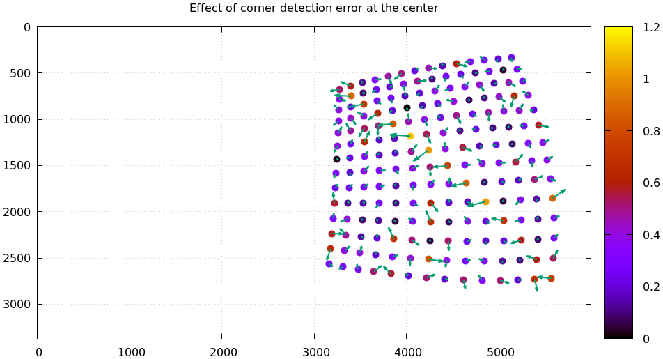
Here we see the residuals on the top-left/bottom-right diagonal be consistently larger than the others, and we see them point in a consistent non-random direction. This isn't easily noticeable without knowing what to look for. But the usual method of zooming in to the worst-few points will make the error in the detected corners visibly apparent.
Rolling shutter
Many cameras employ a rolling shutter: the images aren't captured all at once, but are built up over time, capturing different parts of the image at different times. If the scene or the camera are moving, this would produce images that violate mrcal's view of the world: that at an instant in time I can describe the full chessboard pose and its observed corners. mrcal does not model rolling shutter effects, so non-static calibration images would cause problems. Today the only way to calibrate rolling-shutter cameras with mrcal is to make sure the cameras and the chessboard are stationary during each image capture.
How do we make sure that no rolling-shutter effects ended up in our data? We look at the residuals. Prior to the dataset used in the tour of mrcal I captured images that used the "silent mode" of the Sony Alpha 7 III camera. I didn't realize that this mode implied a rolling shutter, so that dataset wasn't useful to demo anything other than the rolling shutter residuals. Looking at the worst few observations:
mrcal-show-residuals-board-observation \
  --from-worst                         \
  --vectorscale 20                     \
  --circlescale 0.5                    \
  splined.cameramodel                  \
  0-3


I'm omitting the 2nd image because it qualitatively looks very similar to the first. Note the patterns. Clearly something is happening, but it varies from image to image, and a warped chessboard isn't likely to explain it. In addition to that, the magnitude of all the errors is dramatically higher than before: the vectors are scaled up 5x less than those in the tour of mrcal.
Synchronization
What if we're calibrating a multi-camera system, and the image synchronization is broken? You should have a hardware sync: a physical trigger wire connected to each camera, with a pulse on that line telling each camera to begin the image capture. If this is missing or doesn't work properly, then a similar issue occurs as with a rolling-shutter: images captured at allegedly a particular instant in time haven't actually been captured completely at that time.
This can be confirmed by recalibrating monocularly, to see if individually the solves converge. And as expected, this can be readily seen in the residuals. A time sync problem means that synced images A and B were supposed to capture a chessboard at some pose \(T\). But since the sync was broken, the chessboard moved, so the chessboard was really at two different poses: \(T_\mathrm{A}\) and \(T_\mathrm{B}\). mrcal was told that there was no motion, so it ends up solving for some compromise transform \(T_\mathrm{mid}\) that splits the difference. So the residuals for image A would point from the observation at \(T_\mathrm{A}\) towards the observation at the compromise pose \(T_\mathrm{mid}\). And the residuals for image B would point in the opposite direction: from the observation at \(T_\mathrm{B}\) towards the observation at the compromise pose \(T_\mathrm{mid}\).
Let's demo this with a little code. I grab the monocular solve from the tour of mrcal, add a second camera with perfect observations and noise, and add the flaw: one of the chessboard observations was erroneously reported for two images in a row. This happened in only one camera of the pair, so a time-sync error resulted. This is a simulation, but as with everything else on this page, I've seen such problems in real life. The incorrect observation is observation 40, frame 20, camera 0.
#!/usr/bin/python3

import sys
import mrcal
import numpy as np
import numpysane as nps

def binocular_from_monocular(optimization_inputs):
    # Assuming monocular calibration. Add second identical camera to the right
    # of the first
    optimization_inputs['intrinsics'] = \
        nps.glue( optimization_inputs['intrinsics'],
                  optimization_inputs['intrinsics'],
                  axis = -2 )
    optimization_inputs['imagersizes'] = \
        nps.glue( optimization_inputs['imagersizes'],
                  optimization_inputs['imagersizes'],
                  axis = -2 )
    optimization_inputs['rt_cam_ref'] = np.array(((0,0,0, -0.1,0,0),), dtype=float)
    i = optimization_inputs['indices_frame_camintrinsics_camextrinsics']
    optimization_inputs['indices_frame_camintrinsics_camextrinsics'] = \
        np.ascontiguousarray( \
          nps.clump(nps.xchg(nps.cat(i, i + np.array((0,1,1),dtype=np.int32)), 0, 1), n=2))

    # optimization_inputs['observations_board'] needs to have the right shape
    # and the right weights. So I just duplicate it
    optimization_inputs['observations_board'] = \
        np.ascontiguousarray( \
          nps.clump(nps.xchg(nps.cat(optimization_inputs['observations_board'],
                                     optimization_inputs['observations_board']),
                             0,1),
                    n=2))
    del optimization_inputs['imagepaths']

def add_imperfection(optimization_inputs):
    iobservation = 40
    iframe,icam_intrinsics,icam_extrinsics = \
        optimization_inputs['indices_frame_camintrinsics_camextrinsics'][iobservation]
    print(f"observation {iobservation} iframe {iframe} icam_intrinsics {icam_intrinsics} is stuck to the previous observation")

    optimization_inputs    ['observations_board'][iobservation,  ...] = \
        optimization_inputs['observations_board'][iobservation-2,...]


model = mrcal.cameramodel('splined.cameramodel')
optimization_inputs = model.optimization_inputs()

binocular_from_monocular(optimization_inputs)
mrcal.make_perfect_observations(optimization_inputs,
                                observed_pixel_uncertainty = 0)
add_imperfection(optimization_inputs)

optimization_inputs['do_apply_outlier_rejection'] = False
mrcal.optimize(**optimization_inputs)

mrcal.cameramodel(optimization_inputs = optimization_inputs,
                  icam_intrinsics     = 0).write('/tmp/sync-error.cameramodel')

for i in range(2):
    mrcal.show_residuals_board_observation(optimization_inputs,
                                           i,
                                           from_worst  = True,
                                           vectorscale = 2,
                                           circlescale = 0.5)


We're plotting the two worst-residual observations, and we clearly see the tell-tale sign of a time-sync error.
As before, we can make these plots from the commandline:
mrcal-show-residuals-board-observation \
    --from-worst                       \
    --vectorscale 2                    \
    --circlescale 0.5                  \
    /tmp/sync-error.cameramodel        \
    --explore                          \
    0-1
Here we passed --explore to drop into a REPL to investigate further, which
gives us another clear indication that we have a time-sync error. The tool
reports some useful diagnostics at the top of the REPL:
The first 10 worst-fitting observations (i_observations_sorted_from_worst[:10])

[41, 40, 97, 94, 95, 38, 99, 96, 98, 39]


The corresponding 10 (iframe, icamintrinsics, icamextrinsics) tuples
(indices_frame_camintrinsics_camextrinsics[i_observations_sorted_from_worst[:10] ]):

[[20  1  0]
 [20  0 -1]
 [48  1  0]
 [47  0 -1]
 [47  1  0]
 [19  0 -1]
 [49  1  0]
 [48  0 -1]
 [49  0 -1]
 [19  1  0]]
Since a time-sync error affects multiple images at the same time, we should see
multiple chessboard observations from the same frame (instant in time) in the
high-residuals list, and we clearly see that above. We corrupted frame 20 camera
0, so it's no longer syncronized with frame 20 camera 1. We expect both of those
observations to fit badly, and we do see that: the
mrcal-show-residuals-board-observation tool says that the worst residual is
from frame 20 camera 1 and the second-worst is frame 20 camera 0. High errors in
multiple cameras in the same frame like this are another tell-tale sign of sync
errors. We can also query the errors themselves in the REPL:
In [1]: err_per_observation[i_observations_sorted_from_worst][:10]
Out[1]:
array([965407.29301702, 864665.95442895,  11840.10373732,   7762.88344105,
         7759.5509593 ,   7618.23632488,   7190.35449443,   6621.34798572,
         6499.23173619,   6039.45522539])
So the two frame-20 sum-of-squares residuals are on the order of \(900,000 \mathrm{pixels}^2\), and the next worst one is ~ 100 times smaller.
Chessboard shape
Since flat chessboards don't exist, mrcal doesn't assume that the observed chessboard is flat. Today it uses a simple parabolic model. It does assume the board shape is constant throughout the whole calibration sequence. So let's run more simulations to test two scenarios:
- The chessboard is slightly non-flat, but in a way not modeled by the solver
- The chessboard shape changes slightly over the course of the chessboard dance
- Unmodeled chessboard shape
As before, we rerun the scenario from the tour of mrcal with perfect observations and perfect, but with a flaw: I use the very slightly parabolic chessboard, but tell mrcal to assume the chessboard is flat. The script is very similar:
#!/usr/bin/python3

import sys
import mrcal
import numpy as np
import numpysane as nps

def add_imperfection(optimization_inputs):
    H,W = optimization_inputs['observations_board'].shape[1:3]
    s   = optimization_inputs['calibration_object_spacing']
    print(f"Chessboard dimensions are {s*(W-1)}m x {s*(H-1)}m")
    print(f"Chessboard deflection at the center is {optimization_inputs['calobject_warp'][0]*1000:.1f}mm , {optimization_inputs['calobject_warp'][1]*1000:.1f}mm in the x,y direction")
    optimization_inputs['calobject_warp'] *= 0.
    optimization_inputs['do_optimize_calobject_warp'] = False


model = mrcal.cameramodel('splined.cameramodel')
optimization_inputs = model.optimization_inputs()

optimization_inputs['calobject_warp'] = np.array((1e-3, -0.5e-3))
mrcal.make_perfect_observations(optimization_inputs)
add_imperfection(optimization_inputs)
mrcal.optimize(**optimization_inputs)

mrcal.show_residuals_board_observation(optimization_inputs,
                                       0,
                                       from_worst  = True,
                                       vectorscale = 200,
                                       circlescale = 0.5)
It says:
Chessboard dimensions are 0.7644m x 0.7644m
Chessboard deflection at the center is 1.0mm , -0.5mm in the x,y direction
And the worst residual image looks like this:

It usually looks similar to the residuals from a poorly-modeled lens (chessboard edges tend to be observed at the edges of the lens). In this solve the residuals all look low-ish at the center, much bigger at the edges, and consistent at the edges.
- Unstable chessboard shape
What if the chessboard flexes a little bit? I redo my solve using a small parabolic deflection at the first half of the sequence and twice as much deformation during the second half.
#!/usr/bin/python3

import sys
import mrcal
import numpy as np
import numpysane as nps

def add_imperfection(optimization_inputs, observed_pixel_uncertainty):
    Nobservations = len(optimization_inputs['observations_board'])
    observations_half = np.array(optimization_inputs['observations_board'][:Nobservations//2,...])

    optimization_inputs['calobject_warp'] *= 2.
    mrcal.make_perfect_observations(optimization_inputs,
                                    observed_pixel_uncertainty = observed_pixel_uncertainty)

    optimization_inputs['observations_board'][:Nobservations//2,...] = observations_half

    H,W = optimization_inputs['observations_board'].shape[1:3]
    s   = optimization_inputs['calibration_object_spacing']
    print(f"Chessboard dimensions are {s*(W-1)}m x {s*(H-1)}m")
    print(f"Chessboard deflection at the center (second half of dataset) is {optimization_inputs['calobject_warp'][0]*1000:.2f}mm , {optimization_inputs['calobject_warp'][1]*1000:.2f}mm in the x,y direction")
    print(f"Chessboard deflection at the center at the first half of the dataset is half of that")


model = mrcal.cameramodel('splined.cameramodel')
optimization_inputs = model.optimization_inputs()

observed_pixel_uncertainty = np.std(mrcal.measurements_board(optimization_inputs).ravel())

optimization_inputs['calobject_warp'] = np.array((1e-3, -0.5e-3))
mrcal.make_perfect_observations(optimization_inputs,
                                observed_pixel_uncertainty = observed_pixel_uncertainty)

add_imperfection(optimization_inputs, observed_pixel_uncertainty)
mrcal.optimize(**optimization_inputs)

print(f"Optimized chessboard deflection at the center is {optimization_inputs['calobject_warp'][0]*1000:.2f}mm , {optimization_inputs['calobject_warp'][1]*1000:.2f}mm in the x,y direction")


mrcal.cameramodel(optimization_inputs = optimization_inputs,
                  icam_intrinsics     = 0).write('/tmp/unstable-chessboard-shape.cameramodel')

mrcal.show_residuals_board_observation(optimization_inputs,
                                       0,
                                       from_worst  = True,
                                       vectorscale = 200,
                                       circlescale = 0.5)
It says:
Chessboard dimensions are 0.7644m x 0.7644m
Chessboard deflection at the center (second half of dataset) is 2.00mm , -1.00mm in the x,y direction
Chessboard deflection at the center at the first half of the dataset is half of that
Optimized chessboard deflection at the center is 1.66mm , -0.79mm in the x,y direction

It looks a bit like the unmodeled chessboard residuals above, but smaller, and more subtle. But lest you think that these small and subtle residuals imply that this doesn't affect the solution, here's the resulting difference in projection:
mrcal-show-projection-diff                   \
  --no-uncertainties                         \
  --radius 500                               \
  --unset key \
  /tmp/unstable-chessboard-shape.cameramodel \
  splined.cameramodel
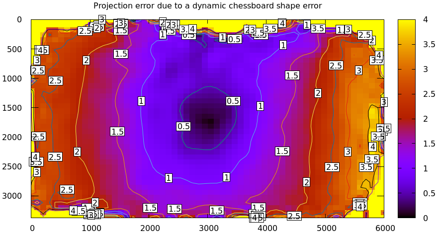
So take care to make your chessboard rigid. I can think of better visualizations to more clearly identify these kinds of issues, so this might improve in the future.
For both of these chessboard deformation cases it's helpful to look at more than just 1 or 2 worst-case residuals. Look at the worst 10. In both cases the most tilted chessboard observations usually show very consistent residual vectors along the far edge of the chessboard.