A tour of mrcal: quantifying uncertainty

It is a reasonable assumption that each \(x\) and \(y\) measurement in every detected chessboard corner contains independent, gaussian noise. This noise is hard to measure directly (there's an attempt in mrgingham), so we estimate it from the solve residuals. We then have the diagonal matrix representing the variance our input noise: \(\mathrm{Var}\left( \vec q_\mathrm{ref} \right)\).

We propagate this input noise through the optimization, to find out how this noise would affect the calibration solution. Given some perturbation of the inputs, we can derive the resulting perturbation in the optimization state: \(\Delta \vec b = M \Delta \vec q_\mathrm{ref}\) for some matrix \(M\) we can compute. The state vector \(\vec b\) contains everything: the intrinsics of all the lenses, the geometry of all the cameras and chessboards, the chessboard shape, etc. We have the variance of the input noise, so we can compute the variance of the state vector:

\[ \mathrm{Var}(\vec b) = M \mathrm{Var}\left(\vec q_\mathrm{ref}\right) M^T \]

Now we need to propagate this uncertainty in the optimization state through a projection. Let's say we have a point \(\vec p_\mathrm{fixed}\) defined in some fixed coordinate system. We need to transform it to the camera coordinate system before we can project it:

\[ \vec q = \mathrm{project}\left( \mathrm{transform}\left( \vec p_\mathrm{fixed} \right)\right) \]

So \(\vec q\) is a function of the intrinsics and the transformation. Both of these are functions of the optimization state, so we can propagate our noise in the optimization state \(\vec b\):

\[ \mathrm{Var}\left( \vec q \right) = \frac{\partial \vec q}{\partial \vec b} \mathrm{Var}\left( \vec b \right) \frac{\partial \vec q}{\partial \vec b}^T \]

There lots and lots of omitted details here, so please read the full documentation if interested.

Let's run some synthetic-data analysis to validate this approach. This all comes directly from the mrcal test suite:

Let's place 4 cameras using a LENSMODEL_OPENCV4 (simple and fast) model side by side, and let's have them look at 50 chessboards, with randomized positions and orientations.

test/test-projection-uncertainty.py \
  --fixed cam0                      \
  --model opencv4                   \
  --do-sample                       \
  --make-documentation-plots ''

The synthetic geometry looks like this:

The solved coordinate system of each camera is shown. Each observed chessboard is shown as a zigzag connecting all the corners in order. The cameras each see:

The purple points are the observed chessboard corners. All the chessboards are roughly at the center of the scene, so the left camera sees objects on the right side of its view, and the right camera sees objects on the left.

We want to evaluate the uncertainty of a calibration made with these observations. So we run 100 randomized trials, where each time we

• add a bit of noise to the observations
• compute the calibration
• look at what happens to the projection of an arbitrary point \(\vec q\) on the imager: the marked \(\color{red}{\ast}\) in the plots above

A confident calibration would have low \(\mathrm{Var}\left(\vec q\right)\), and projections would be insensitive to observation noise: the \(\color{red}{\ast}\) wouldn't move much as we add input noise. By contrast, a poor calibration would have high uncertainty, and the \(\color{red}{\ast}\) would move significantly due to random observation noise.

The above command runs the trials, following the reprojection of \(\color{red}{\ast}\). We plot the empirical 1-sigma ellipse computed from these samples, and also the 1-sigma ellipse predicted by the mrcal.projection_uncertainty() routine. This is the routine that implements the scheme described above, but does so analytically, without any sampling. It is thus much faster.

Clearly the two ellipses (blue and green) line up well, so there's good agreement between the observed and predicted uncertainties. So from now on we will use the predictions only.

We see that the reprojection uncertainties of this point are different for each camera. This happens because the distribution of chessboard observations is different in each camera. We're looking at a point in the top-left quadrant of the imager. And as we saw before, this point was surrounded by chessboard observations only in the first camera. In the second and third cameras, this point was on the edge of region of chessboard observations. And in the last camera, the observations were all quite far away from this query point. In that camera, we have no data about the lens behavior in this area, and we're extrapolating. We should expect to have the best uncertainty in the first camera, worse uncertainties in the next two cameras, and poor uncertainty in the last camera. And this is exactly what we observe.

Now that we validated the relatively quick-to-compute mrcal.projection_uncertainty() estimates, let's use them to compute uncertainty maps across the whole imager, not just at a single point:

As expected, we see that the sweet spot is different for each camera, and it tracks the location of the chessboard observations. And we can see that the \(\color{red}{\ast}\) is in the sweet spot only in the first camera.

Let's focus on the last camera. Here the chessboard observations were nowhere near the focus point, and we reported an expected reprojection error of ~0.8 pixels. This is significantly worse than the other cameras, but it's not terrible in absolute terms. If an error of 0.8 pixels is acceptable for our application, could we use that calibration result to project points around the \(\color{red}{\ast}\)?

Unfortunately, we cannot. We didn't observe any chessboards there, so we don't know how the lens behaves in that area. The optimistic result reported by the uncertainty algorithm isn't wrong, but it's not answering the question we're asking. We're computing how observation noise affects the whole optimizer state, including the lens parameters (LENSMODEL_OPENCV4 in this case). And then we compute how the noise in those lens parameters and geometry affects projection. The LENSMODEL_OPENCV4 model is very lean (has few parameters). This gives it stiffness, which prevents the projection \(\vec q\) from moving very far in response to noise, which we then interpret as a relatively-low uncertainty of 0.8 pixels. If we used a model with more parameters, the extra flexibility would allow the projection to move much further in response to noise, and we'd see a higher uncertainty. So here our choice of lens model itself is giving us low uncertainties. If we knew for a fact that the true lens is 100% representable by a LENSMODEL_OPENCV4 model, then this would be be correct, but that never happens in reality. So lean models always produce overly-optimistic uncertainty estimates.

This is yet another advantage of splined models: they're flexible, so the model itself has little effect on the reported uncertainty. And we get the behavior we want: reported uncertainty is driven only by the data we have gathered.

Let's re-run this analysis using a splined model, and let's look at the same uncertainty plots as above (note: this is slow):

test/test-projection-uncertainty.py \
  --fixed cam0                      \
  --model splined                   \
  --do-sample                       \
  --make-documentation-plots ''

As expected, the reported uncertainties are now far worse. In fact, we can see that only the first camera's projection is truly reliable at the \(\color{red}{\ast}\). This is representative of reality.

To further clarify where the uncertainty region comes from, let's overlay the chessboard observations onto it:

The connection between the usable-projection region and the observed-chessboards region is indisputable. This plot also sheds some light on the effects of spline density. If we had a denser spline, some of the gaps in-between the chessboard observations would show up as poor-uncertainty regions. This hasn't yet been studied on real-world data.

Given this, I claim that we want to use splined models in most situations, even for long lenses which roughly follow the pinhole model. The basis of mrcal's splined models is the stereographic projection, which is identical to a pinhole projection when representing a long lens, so the splined models will also fit long lenses well. The only downside to using a splined model in general is the extra required computational cost. It isn't terrible today, and will get better with time. And for that low price we get the extra precision (no lens follows the lean models when you look closely enough) and we get truthful uncertainty reporting.

We started this by calibrating a camera using a LENSMODEL_OPENCV8 model, and then again with a splined model. Let's look at the uncertainty of those solves using the handy mrcal-show-projection-uncertainty tool.

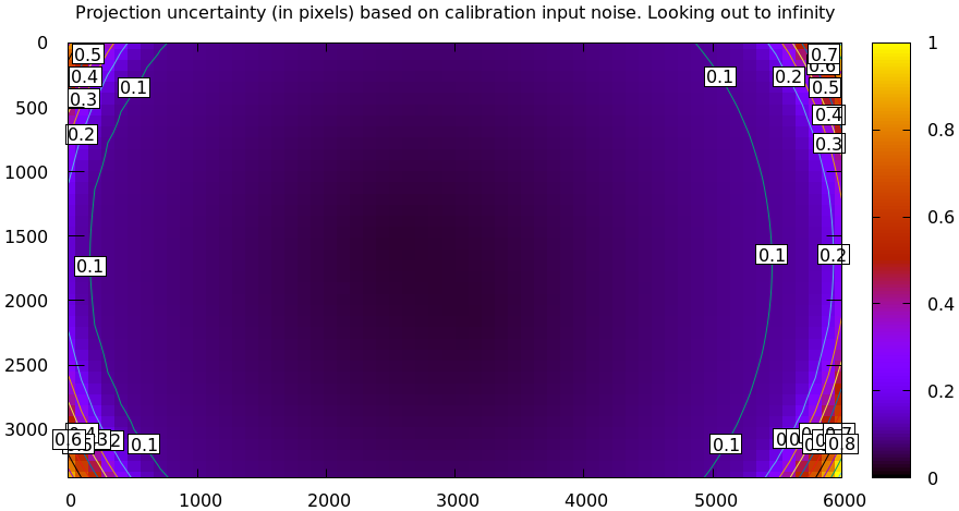
First, the LENSMODEL_OPENCV8 solve:

mrcal-show-projection-uncertainty opencv8.cameramodel --cbmax 1 --unset key

And the splined solve:

mrcal-show-projection-uncertainty splined.cameramodel --cbmax 1 --unset key

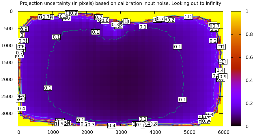
As expected, the splined model produces less optimistic (but more realistic) uncertainty reports.

In the last section we compared our two calibrated models, and the difference looked like this:

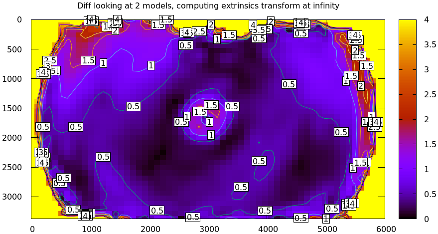
Clearly the errors predicted by the projection uncertainty plots don't account for the large differences we see here: roughly we want to see \(\mathrm{difference} \approx \mathrm{uncertainty}_0 + \mathrm{uncertainty}_1\). The reason for this is non-negligible model errors, so this is a good time to talk about cross-validation.