A tour of mrcal
Table of Contents
mrcal is a general-purpose toolkit that can solve a number of problems. The best way to convey a sense of the capabilities is to demonstrate some real-world usage scenarios. So let's go through a full calibration sequence starting with chessboard images, and eventually finishing with stereo processing. This page is a high-level overview; for more details, please see the main documentation.
All images have been gathered with a Nikon D750 SLR. I want to stress-test the system, so I'm using the widest lens I can find: a Samyang 12mm F2.8 fisheye lens. This lens has a ~ 180deg field of view corner to corner, and about 150deg field of view horizontally.
In these demos I'm using only one camera, so I'm going to run a monocular calibration to compute the intrinsics (the lens parameters). mrcal is fully able to calibrate any N cameras at a time, I'm just using the one camera here.
Gathering chessboard corners
We start by gathering images of a chessboard. This is a wide lens, so I need a large chessboard in order to fill the imager. My chessboard has 10x10 internal corners with a corner-corner spacing of 7.7cm. A big chessboard such as this is never completely rigid or completely flat. I'm using a board backed with 2cm of foam, which keeps the shape stable over short periods of time, long-enough to complete a board dance. But the shape still drifts with changes in temperature and humidity, so mrcal estimates the board shape as part of its calibration solve.
An important consideration when gathering calibration images is keeping them in focus. As we shall see later, we want to gather close-up images as much as possible, so depth-of-field is the limiting factor. Moving the focus ring or the aperture ring on the lens may affect the intrinsics, so ideally a single lens setting can cover both the calibration-time closeups and the working distance (presumably much further out).
So for these tests I set the focus to infinity, and gather all my images at F22 to increase the depth-of-field as much as I can. To also avoid motion blur I need fast exposures, so I did all the image gathering outside, with bright natural lighting.
The images live here. I'm using mrgingham 1.17 to detect the chessboard corners:
mrgingham -j3 '*.JPG' > corners.vnl
How well did we cover the imager? Did we get the edges and corners?
$ < corners.vnl       \
  vnl-filter -p x,y | \
  feedgnuplot --domain --square --set 'xrange [0:6016]' --set 'yrange [4016:0]'
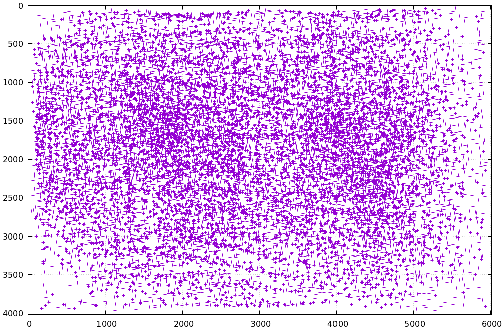
Looks like we did OK. It's a bit thin along the bottom edge, but not terrible. For an arbitrary image we can visualize at the corner detections:
$ < corners.vnl head -n5

## generated with mrgingham -j3 *.JPG
# filename x y level
DSC_7374.JPG 1049.606126 1032.249784 1
DSC_7374.JPG 1322.477977 1155.491028 1
DSC_7374.JPG 1589.571471 1276.563664 1


$ f=DSC_7374.JPG

$ < corners.vnl \
    vnl-filter "filename eq \"$f\"" --perl -p x,y,size='2**(1-level)' | \
  feedgnuplot --image $f --domain --square --tuplesizeall 3 \
              --with 'points pt 7 ps variable'
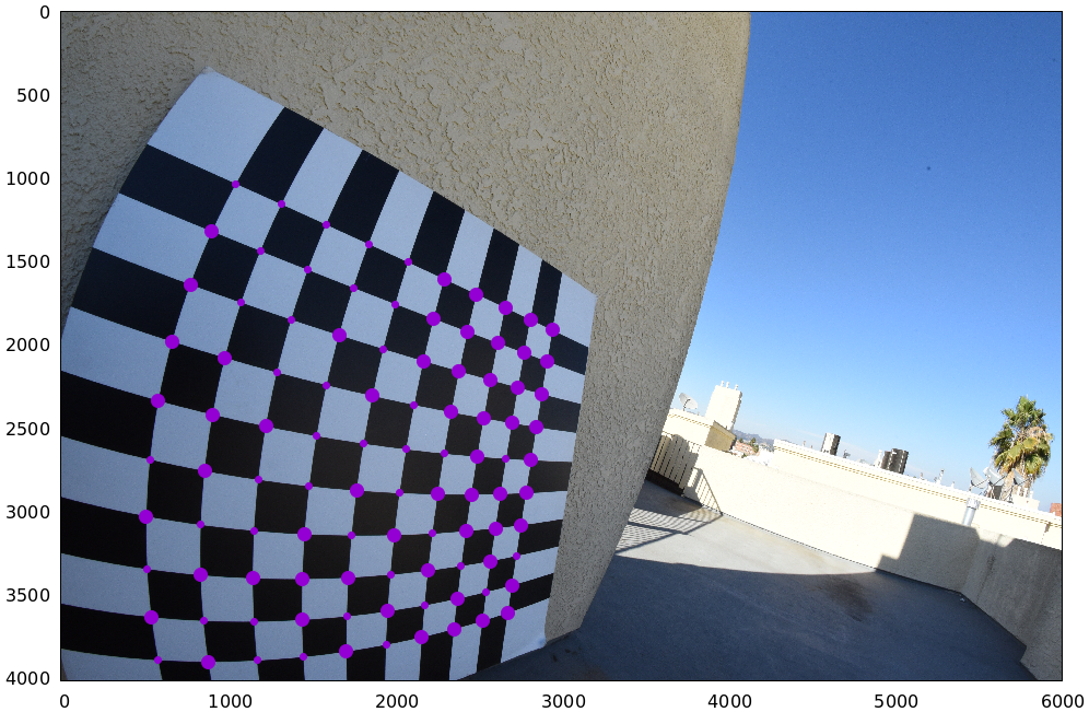
So in this image many of the corners were detected at full-resolution (level-0), but some required downsampling for the detector to find them: shown as smaller circles. The downsampled points have less precision, so they are weighed less in the optimization. How many images produced successful corner detections?
$ < corners.vnl vnl-filter --has x -p filename | uniq | grep -v '#' | wc -l

186


$ < corners.vnl vnl-filter x=='"-"' -p filename | uniq | grep -v '#' | wc -l

89
So we have 186 images with detected corners, and 89 images where a full chessboard wasn't found. Most of the misses are probably images where the chessboard wasn't entirely in view, but some could be failures of mrgingham. In any case, 186 observations is usually plenty.
If I had more that one camera, the image filenames would need to indicate what
camera captured each image at which time. I generally use
frameFFF-cameraCCC.jpg. Images with the same FFF are assumed to have been
captured at the same instant in time.
Monocular calibration with the 8-parameter opencv model
Let's calibrate the intrinsics! We begin with LENSMODEL_OPENCV8, a lean model
that supports wide lenses decently well. Primarily it does this with a rational
radial "distortion" model. Projecting \(\vec p\) in the camera coordinate system:
Where \(\vec q\) is the resulting projected pixel, \(\vec f_{xy}\) is the focal lengths and \(\vec c_{xy}\) is the center pixel of the imager.
Let's compute the calibration: the mrcal-calibrate-cameras tool is the main
frontend for that purpose.
$ mrcal-calibrate-cameras        \
  --corners-cache corners.vnl    \
  --lensmodel LENSMODEL_OPENCV8  \
  --focal 1700                   \
  --object-spacing 0.077         \
  --object-width-n 10            \
  --observed-pixel-uncertainty 2 \
  --explore                      \
  '*.JPG'


vvvvvvvvvvvvvvvvvvvv initial solve: geometry only
^^^^^^^^^^^^^^^^^^^^ RMS error: 32.19393243308936

vvvvvvvvvvvvvvvvvvvv initial solve: geometry and intrinsic core only
^^^^^^^^^^^^^^^^^^^^ RMS error: 12.308083539621899
=================== optimizing everything except board warp from seeded intrinsics
mrcal.c(4974): Threw out some outliers (have a total of 3 now); going again
vvvvvvvvvvvvvvvvvvvv final, full re-optimization call to get board warp
^^^^^^^^^^^^^^^^^^^^ RMS error: 0.7809749790209548
RMS reprojection error: 0.8 pixels
Worst residual (by measurement): 7.2 pixels
Noutliers: 3 out of 18600 total points: 0.0% of the data
calobject_warp = [-0.00103983  0.00052493]

Wrote ./camera-0.cameramodel
The resulting model is available here. This is a mrcal-native .cameramodel
file containing at least the lens parameters and the geometry. For uncertainty
quantification and for after-the-fact analysis, the full optimization inputs
are included in this file. Reading and re-optimizing those inputs is trivial:
import mrcal

m = mrcal.cameramodel('camera-0.cameramodel')
optimization_inputs = m.optimization_inputs()
mrcal.optimize(**optimization_inputs)
model_reoptimized = \
  mrcal.cameramodel( optimization_inputs = m.optimization_inputs(),
                     icam_intrinsics     = m.icam_intrinsics() )
model_reoptimized.write('camera0-reoptimized.cameramodel')
Here we didn't make any changes to the inputs, and we should already have an optimal solution, so the re-optimized model is the same as the initial one. But we could add input noise or change the lens model or regularization terms or anything else, and we would then observe the effects of those changes.
I'm specifying the initial very rough estimate of the focal length (in pixels),
the geometry of my chessboard (10x10 board with 0.077m spacing between corners),
the lens model I want to use, chessboard corners we just detected, the estimated
uncertainty of the corner detections (more on this later) and the image globs. I
have just one camera, so I have one glob: *.JPG. With more cameras you'd have
something like '*-camera0.jpg' '*-camera1.jpg' '*-camera2.jpg'.
--explore asks the tool to drop into a REPL after it's done computing so that
we can look around. Most visualizations can be made by running the
mrcal-show-... commandline tools on the generated xxx.cameramodel files, but
some of the residual visualizations are only available inside the REPL at this
time.
The --observed-pixel-uncertainty is a rough estimate of the input pixel noise,
used primarily for the projection uncertainty reporting.
Let's sanity-check the results. We want to flag down any issues with the data that would violate the assumptions made by the solver.
The tool reports some diagnostics. As we can see, the final RMS reprojection error was 0.8 pixels. Of the 18600 corner observations (186 observations of the board with 10*10 = 100 points each), 3 didn't fit the model well, and were thrown out as outliers. And the board flex was computed as 1.0mm horizontally, and 0.5mm vertically in the opposite direction. That all sounds reasonable.
What does the solve think about our geometry? Does it match reality?
show_geometry( _set  = ('xyplane 0', 'view 80,30,1.5'),
               unset = 'key')
We could also have used the mrcal-show-geometry tool from the shell. All plots
are interactive when executed from the REPL or from the shell. Here we see the
axes of our camera (purple) situated in the reference coordinate system. In this
solve, the camera coordinate system is the reference coordinate system; this
would look more interesting with more cameras. In front of the camera (along the
\(z\) axis) we can see the solved chessboard poses. There are a whole lot of them,
and they're all sitting right in front of the camera with some heavy tilt. This
matches with how this chessboard dance was performed (it was performed following
the guidelines set by the dance study).
Next, let's examine the residuals more closely. We have an overall RMS reprojection-error value from above, but let's look at the full distribution of errors for all the cameras:
show_residuals_histogram(icam = None, binwidth=0.1, _xrange=(-4,4), unset='key')
We would like to see a normal distribution since that's what the noise model
assumes. We do see this somewhat, but the central cluster is a bit
over-populated. Not a ton to do about that, so I will claim this is
close-enough. We see the normal distribution fitted to our data, and we see the
normal distribution as predicted by the --observed-pixel-uncertainty. Our
error distribution fits tighter than the distribution predicted by the input
noise. This is expected for two reasons:
- We don't actually know what
--observed-pixel-uncertaintyis; the value we're using is a rough estimate - We're overfitting. If we fit a model using just a little bit of data, we would overfit, the model would explain the noise in the data, and we would get very low fit errors. As we get more and more data, this effect is reduced, and eventually the data itself drives the solution, and the residual distribution matches the distribution of input noise. Here we never quite get there. But this isn't a problem: we explicitly quantify our uncertainty, so while we do see some overfitting, we know exactly how much it affects the reliability of our results. And we can act on that information.
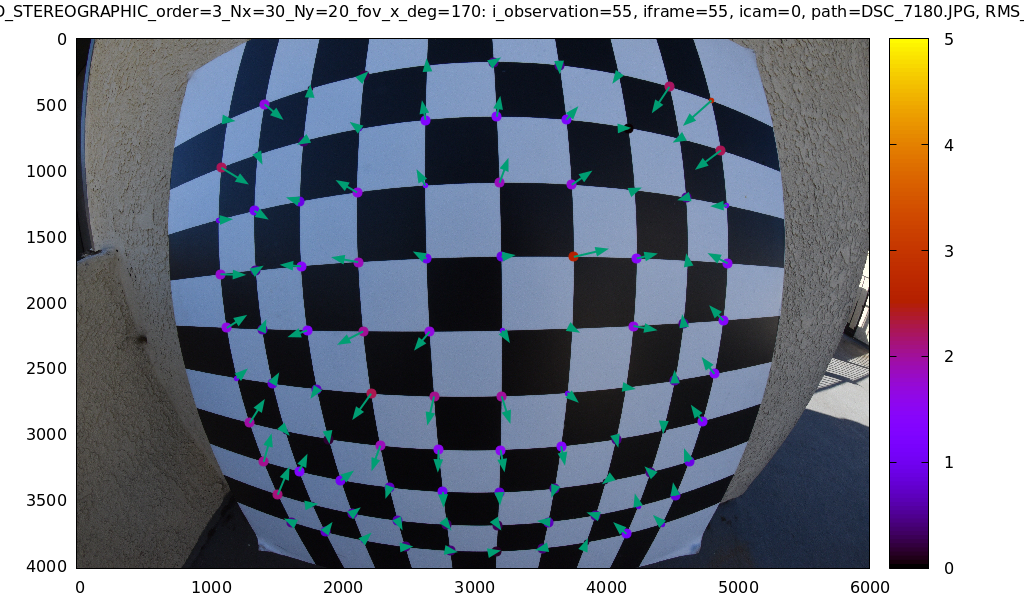
Let's look deeper. If there's anything really wrong with our data, then we should see it in the worst-fitting images. Let's ask the tool to see the worst one:
show_residuals_observation_worst(0, vectorscale = 100, circlescale=0.5,
                                 cbmax = 5.0)
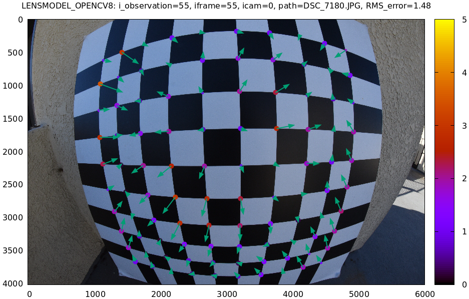
The residual vector for each chessboard corner in this observation is shown, scaled by a factor of 100 for legibility (the actual errors are tiny!) The circle color also indicates the magnitude of the errors. The size of each circle represents the weight given to that point. The weight is reduced for points that were detected at a lower resolution by the chessboard detector. Points thrown out as outliers are not shown at all.
This is the worst-fitting image, so any data-gathering issues will show up in this plot.
We look for any errors that look unreasonably large. And we look for patterns. In a perfect world, the model fits the observations, and the residuals display purely random noise. Any patterns in the errors indicate that the noise isn't random, and thus the model does not fit. This would violate the noise model, and would result in a bias when we ultimately use this calibration for projection. This bias is an unmodeled source of error, so we really want to push this down as far as we can. Getting rid of all such errors completely is usually impossible, but we should do our best.
Common sources of unmodeled errors:
- out-of focus images
- images with motion blur
- rolling shutter effects
- synchronization errors
- chessboard detector failures
- insufficiently-rich models (of the lens or of the chessboard shape or anything else)
Back to this image. In absolute terms, even this worst-fitting image fits really well. The RMS error of the errors in this image is 1.48 pixels. The residuals in this image look mostly reasonable. There is a bit of a pattern: errors point outwardly in the center, larger errors on the outside of the image, pointing mostly inward. This isn't great, but it's a small effect, so let's keep going.
One issue with lean models such as LENSMODEL_OPENCV8 is that the radial
distortion is never quite right, especially as we move further and further away
form the optical axis: this is the last point in the common-errors list above.
We can clearly see this here in the 3rd-worst image:
show_residuals_observation_worst(2, vectorscale = 100, circlescale=0.5,
                                 cbmax = 5.0)
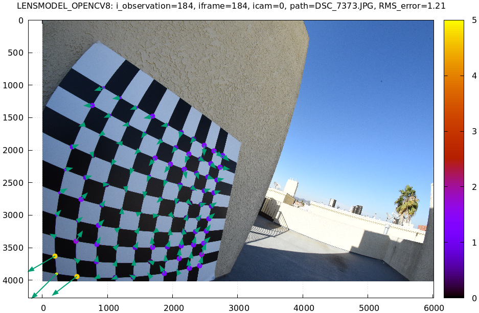
This is clearly a problem. Which observation is this, so that we can come back to it later?
print(i_observations_sorted_from_worst[2])

---> 184
Let's look at the systematic errors in another way: let's look at all the residuals over all the observations, color-coded by their direction, ignoring the magnitudes:
show_residuals_directions(icam=0, unset='key', valid_intrinsics_region = False)
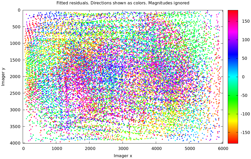
As before, if the model fit the observations, the errors would represent random noise, and no color pattern would be discernible in these dots. Here we can clearly see lots of green in the top-right and top and left, lots of blue and magenta in the center, yellow at the bottom, and so on. This is not random noise, and is a very clear indication that this lens model is not able to fit this data.
It would be very nice to have a quantitative measure of these systematic patterns. At this time mrcal doesn't provide an automated way to do that.
Clearly there're unmodeled errors in this solve. As we have seen, the errors here are all fairly small, but they become very important when doing precision work like, for instance, long-range stereo.
Let's fix it.
Monocular calibration with a splined stereographic model
Usable uncertainty quantification and accurate projections are major goals of mrcal. To achive these, mrcal supports splined models. At this time there's only one representation supported: a splined stereographic model, described in detail here.
Splined stereographic model definition
The basis of a splined stereographic model is a stereographic projection. In this projection, a point that lies an angle \(\theta\) off the camera's optical axis projects to \(\left|\vec q - \vec q_\mathrm{center}\right| = 2 f \tan \frac{\theta}{2}\) pixels from the imager center, where \(f\) is the focal length. Note that this representation supports projections behind the camera (\(\theta > 90^\circ\)) with a single singularity directly behind the camera. This is unlike the pinhole model, which has \(\left|\vec q - \vec q_\mathrm{center}\right| = f \tan \theta\), and projects to infinity as \(\theta \rightarrow 90^\circ\).
Basing the new model on a stereographic projection lifts the inherent
forward-view-only limitation of LENSMODEL_OPENCV8. To give the model enough
flexibility to be able to represent any projection function, I define two
correction surfaces.
Let \(\vec p\) be the camera-coordinate system point being projected. The angle off the optical axis is
\[ \theta \equiv \tan^{-1} \frac{\left| \vec p_{xy} \right|}{p_z} \]
The normalized stereographic projection is
\[ \vec u \equiv \frac{\vec p_{xy}}{\left| \vec p_{xy} \right|} 2 \tan\frac{\theta}{2} \]
This initial projection operation unambiguously collapses the 3D point \(\vec p\) into a 2D point \(\vec u\). We then use \(\vec u\) to look-up an adjustment factor \(\Delta \vec u\) using two splined surfaces: one for each of the two elements of
\[ \Delta \vec u \equiv \left[ \begin{aligned} \Delta u_x \left( \vec u \right) \\ \Delta u_y \left( \vec u \right) \end{aligned} \right] \]
We can then define the rest of the projection function:
\[\vec q = \left[ \begin{aligned} f_x \left( u_x + \Delta u_x \right) + c_x \\ f_y \left( u_y + \Delta u_y \right) + c_y \end{aligned} \right] \]
The parameters we can optimize are the spline control points and \(f_x\), \(f_y\), \(c_x\) and \(c_y\), the usual focal-length-in-pixels and imager-center values.
Solving
Let's run the same exact calibration as before, but using the richer model to specify the lens:
$ mrcal-calibrate-cameras                                                       \
  --corners-cache corners.vnl                                                   \
  --lensmodel LENSMODEL_SPLINED_STEREOGRAPHIC_order=3_Nx=30_Ny=20_fov_x_deg=170 \
  --focal 1700                                                                  \
  --object-spacing 0.077                                                        \
  --object-width-n 10                                                           \
  --observed-pixel-uncertainty 2                                                \
  --explore                                                                     \
  '*.JPG'


vvvvvvvvvvvvvvvvvvvv initial solve: geometry only
^^^^^^^^^^^^^^^^^^^^ RMS error: 32.19393243308936

vvvvvvvvvvvvvvvvvvvv initial solve: geometry and intrinsic core only
^^^^^^^^^^^^^^^^^^^^ RMS error: 12.308083539621899
=================== optimizing everything except board warp from seeded intrinsics
vvvvvvvvvvvvvvvvvvvv final, full re-optimization call to get board warp
^^^^^^^^^^^^^^^^^^^^ RMS error: 0.599580146623648
RMS reprojection error: 0.6 pixels
Worst residual (by measurement): 4.3 pixels
Noutliers: 0 out of 18600 total points: 0.0% of the data
calobject_warp = [-0.00096895  0.00052931]
The resulting model is available here.
The lens model
LENSMODEL_SPLINED_STEREOGRAPHIC_order=3_Nx=30_Ny=20_fov_x_deg=170 is the only
difference in the command. Unlike LENSMODEL_OPENCV8, this model has some
configuration parameters: the spline order (we use cubic splines here), the
spline density (here each spline surface has 30 x 20 knots), and the rough
horizontal field-of-view we support (we specify about 170 degrees horizontal
field of view).
There're over 1000 lens parameters here, but the problem is very sparse, so we can still process this in a reasonable amount of time.
The LENSMODEL_OPENCV8 solve had 3 points that fit so poorly, the solver threw them away as
outliers. Here we have 0. The RMS reprojection error dropped from 0.8 pixels to
0.6. The estimated chessboard shape stayed roughly the same. These are all what
we hope to see.
Let's look at the residual distribution in this solve:
show_residuals_histogram(0, binwidth=0.1, _xrange=(-4,4), unset='key')
This still has the nice bell curve, but the residuals are lower: the data fits better than before.
Let's look at the worst-fitting single image in this solve:
show_residuals_observation_worst(0, vectorscale = 100, circlescale=0.5,
                                 cbmax = 5.0)
Interestingly, the worst observation here is the same one we saw with
LENSMODEL_OPENCV8. But all the errors are significantly smaller than before.
The previous pattern is much less pronounced, but it still there. I don't know
the cause conclusively. My suspicion is that the board flex model isn't quite
rich-enough. In any case, these errors are small, so let's proceed.
What happens when we look at the image that showed a poor fit in the corner previously? It was observation 184.
show_residuals_observation(184, vectorscale = 100, circlescale=0.5,
                           cbmax = 5.0)
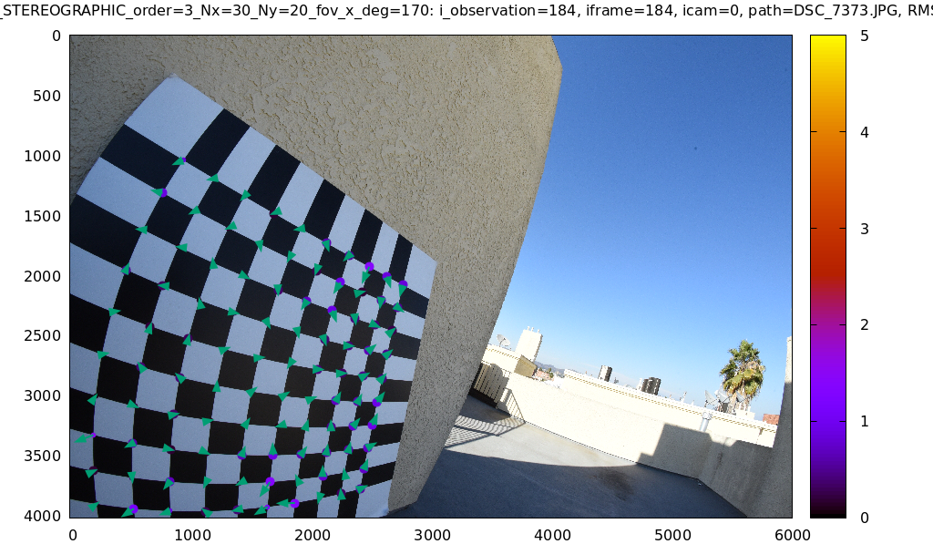
Neat! The model fits the data in the corners now. And what about the residual directions?
show_residuals_directions(icam=0, unset='key', valid_intrinsics_region = False)
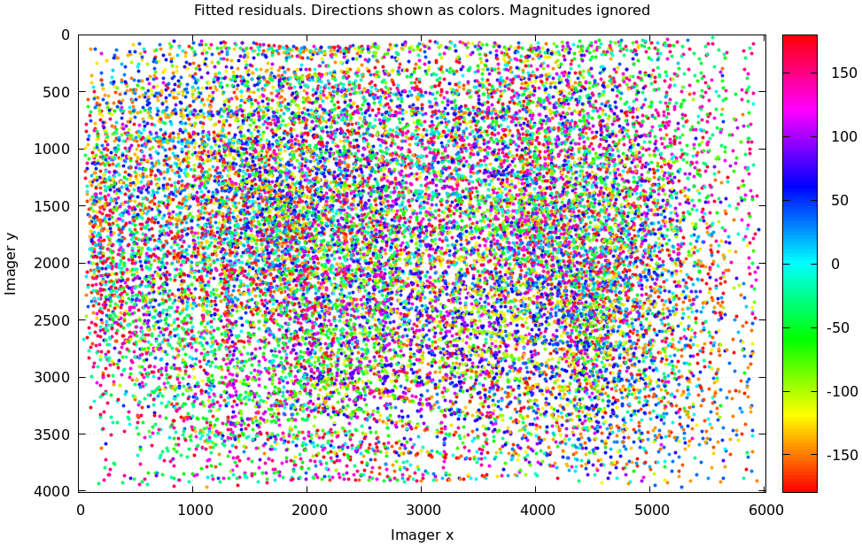
Much better than before. Maybe there's still a pattern, but it's not clearly discernible.
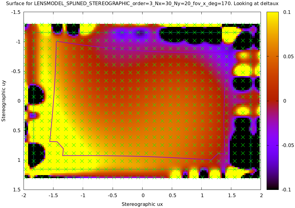
We can also visualize the splined surfaces themselves. Here I'm using the
commandline tool instead of a function in the mrcal-calibrate-cameras REPL.
mrcal-show-splined-model-surface splined.cameramodel x \
                                 --set 'cbrange [-.1:.1]' --unset key

mrcal-show-splined-model-surface splined.cameramodel y \
                                 --set 'cbrange [-.1:.1]' --unset key
\(\Delta u_x\) looks like this:
And \(\Delta u_y\):
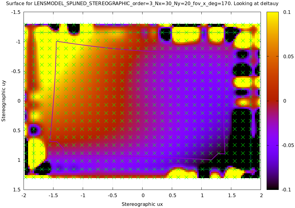
Each X in the plot is a "knot" of the spline surface, a point where a control point value is defined. We're looking at the spline domain, so the axes of the plot are \(u_x\) and \(u_y\), and the knots are arranged in a regular grid. The region where the spline surface is well-defined begins at the 2nd knot from the edges; its boundary is shown as a thin green line. The valid-intrinsics region (the area where the intrinsics are confident because we had lots of chessboard observations there) is shown as a thick, purple curve. Since each \(\vec u\) projects to a pixel coordinate \(\vec q\) in some very nonlinear way, this curve is very much not straight.
We want the valid-intrinsics region to lie entirely within the spline-in-bounds region, and that happens here. If some observations lie outside the spline-in-bounds regions, the projection behavior at the edges will be less flexible than the rest of the model, resulting in less realistic uncertainties there. See the lensmodel documentation for more detail.
Alternately, I can look at the spline surface as a function of the pixel coordinates. Just for \(\Delta u_x\):
mrcal-show-splined-model-surface splined.cameramodel x                \
                                 --imager-domain                      \
                                 --set 'cbrange [-.1:.1]' --unset key \
                                 --set 'xrange [-300:6300]'           \
                                 --set 'yrange [4300:-300]'
![]()
Now the valid-intrinsics region is a nice rectangle, but the spline-in-bounds region is complex curve. Projection at the edges is poorly-defined, so the boundary of the spline-in-bounds region appears highly irregular in this view.
This scary-looking behavior is a side-effect of the current representation, but it is benign: the questionable projections lie in regions where we have no expectation of a reliable projection.
Differencing
An overview follows; see the differencing page for details.
We just used the same chessboard observations to compute the intrinsics of a lens in two different ways:
- Using a lean
LENSMODEL_OPENCV8lens model - Using a rich splined-stereographic lens model
And we saw evidence that the splined model does a better job of representing reality. Can we quantify that? How different are the two models we computed?
Let's compute the difference. Given a pixel \(\vec q_0\) we can
- Unproject \(\vec q_0\) to a fixed point \(\vec p\) using lens 0
- Project \(\vec p\) back to pixel coords \(\vec q_1\) using lens 1
- Report the reprojection difference \(\vec q_1 - \vec q_0\)
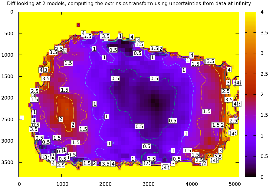
This is a very common thing to want to do, so mrcal provides a tool to do it. Let's compare the two models:
mrcal-show-projection-diff --radius 0 --cbmax 200 --unset key \
                           opencv8.cameramodel splined.cameramodel
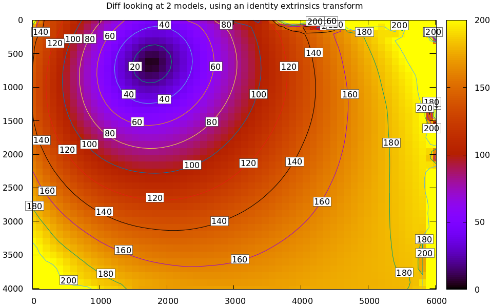
Well that's strange. The reported differences really do have units of pixels. Are the two models that different? And is the best-aligned area really where this plot indicates? If we ask for the vector field of differences instead of a heat map, we get a hint about what's going on:
mrcal-show-projection-diff --radius 0 --cbmax 200 --unset key \
                           --vectorfield --vectorscale 5 --gridn 30 20 \
                           opencv8.cameramodel splined.cameramodel
This is a very regular pattern. What does it mean?
The issue is that each calibration produces noisy estimates of all the intrinsics and all the coordinate transformations:
The above plots projected the same \(\vec p\) in the camera coordinate system, but that coordinate system has shifted between the two models we're comparing. So in the fixed coordinate system attached to the camera housing, we weren't in fact projecting the same point.
There exists some transformation between the camera coordinate system from the solution and the coordinate system defined by the physical camera housing. It is important to note that this implied transformation is built-in to the intrinsics. Even if we're not explicitly optimizing the camera pose, this implied transformation is still something that exists and moves around in response to noise. Rich models like the splined stereographic models are able to encode a wide range of implied transformations, but even the simplest models have some transform that must be compensated for.
The above vector field suggests that we need to move one of the cameras up and to the left, and then we need to rotate that camera. We can automate this by adding a critical missing step to the procedure above between steps 1 and 2:
- Transform \(\vec p\) from the coordinate system of one camera to the coordinate system of the other camera
But we don't know anything about the physical coordinate system of either
camera. How can we compute this transformation? We do a fit. The "right"
transformation will transform \(\vec p\) in such a way that the reported
mismatches in \(\vec q\) will be minimized. Lots of details are glossed-over here.
Previously we passed --radius 0 to bypass the fit. Let's leave out that option
to get the usable diff:
mrcal-show-projection-diff --unset key \
                           opencv8.cameramodel splined.cameramodel
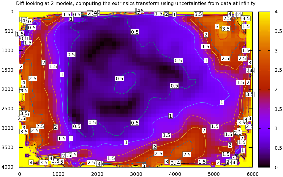
Much better. As expected, the two models agree relatively well in the center,
and the error grows as we move towards the edges. If we used a leaner model,
such as LENSMODEL_OPENCV4, this effect would be far more pronounced:
mrcal-show-projection-diff --no-uncertainties \
  --distance 1 --radius 200 \
  --unset key --extratitle "radius 200" opencv[48].cameramodel
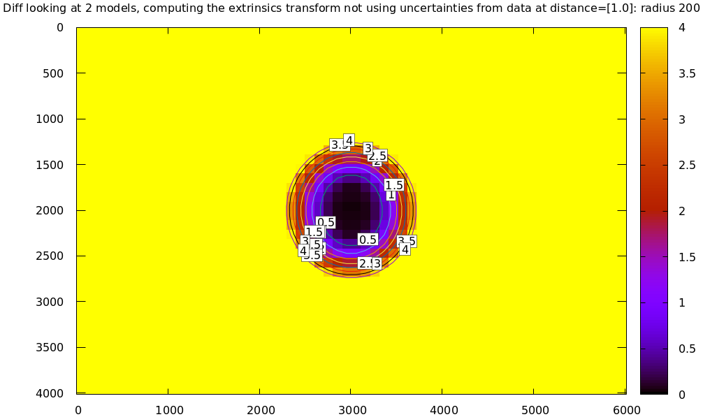
Please see the differencing page for details.
This differencing method is very powerful, and has numerous applications. For instance:
- evaluating the manufacturing variation of different lenses
- quantifying intrinsics drift due to mechanical or thermal stresses
- testing different solution methods
- underlying a cross-validation scheme
Many of these analyses immediately raise a question: how much of a difference do I expect to get from random noise, and how much is attributable to whatever I'm measuring?
Furthermore, how do we decide which data to use for the fit of the implied transformation? Here I was careful to get chessboard images everywhere in the imager, but what if there was occlusion in the space, so I was only able to get images in one area? In this case we would want to use only the data in that area for the fit of the implied transformation (because we won't expect the data in other areas to fit). But what to do if we don't know where that area is?
These questions can be answered conclusively by quantifying the projection uncertainty, so let's talk about that now.
Projection uncertainty
An overview follows; see the noise model and projection uncertainty pages for details.
It would be really nice to be able to compute an uncertainty along with every projection operation: given a camera-coordinate point \(\vec p\) we would compute the projected pixel coordinate \(\vec q\), along with the covariance \(\mathrm{Var} \left(\vec q\right)\) to represent the uncertainty. If this were available we could
- Propagate this uncertainty downstream to whatever uses the projection operation, for example to get the uncertainty of ranges from a triangulation
- Evaluate how trustworthy a given calibration is, and to run studies about how to do better
- Quantify overfitting effects
- Quantify the baseline noise level for informed interpretation of model differences
- Intelligently select the region used to compute the implied transformation when computing differences
These are quite important. Since splined models can have 1000s of parameters, we will overfit when using those models. This isn't a problem in itself, however. "Overfitting" simply means the uncertainty is higher than it otherwise would be. And if we can quantify that uncertainty, we can decide if we have too much.
Derivation summary
It is a reasonable assumption that each \(x\) and \(y\) measurement in every detected chessboard corner contains independent, gaussian noise. This noise is hard to measure (there's an attempt in mrgingham), but easy to loosely estimate. The current best practice is to get a conservative eyeball estimate to produce conservative estimates of projection uncertainty. So we have the diagonal matrix representing the variance our input noise: \(\mathrm{Var}\left( \vec q_\mathrm{ref} \right)\).
We then propagate this input noise through the optimization, to find out how this noise would affect the calibration solution. Given some perturbation of the inputs, we can derive the resulting perturbation in the optimization state: \(\Delta \vec p = M \Delta \vec q_\mathrm{ref}\) for some matrix \(M\) we can compute. The state vector \(\vec p\) contains everything: the intrinsics of all the lenses, the geometry of all the cameras and chessboards, the chessboard shape, etc. We have the variance of the input noise, so we can compute the variance of the state vector:
\[ \mathrm{Var}(\vec p) = M \mathrm{Var}\left(\vec q_\mathrm{ref}\right) M^T \]
Now we need to propagate this uncertainty in the optimization state through a projection. Let's say we have a point \(\vec p_\mathrm{fixed}\) defined in some fixed coordinate system. We need to transform it to the camera coordinate system before we can project it:
\[ \vec q = \mathrm{project}\left( \mathrm{transform}\left( \vec p_\mathrm{fixed} \right)\right) \]
So \(\vec q\) is a function of the intrinsics, and the transformation. Both of these are functions of the optimization state, so we can propagate our noise in the optimization state \(\vec p\):
\[ \mathrm{Var}\left( \vec q \right) = \frac{\partial \vec q}{\partial \vec p} \mathrm{Var}\left( \vec p \right) \frac{\partial \vec q}{\partial \vec p}^T \]
There lots and lots of details here, so please read the documentation if interested.
Simulation
Let's run some synthetic-data analysis to validate this approach. This all comes directly from the mrcal test suite:
test/test-projection-uncertainty.py --fixed cam0 --model opencv4 \
                                    --make-documentation-plots
Let's place 4 cameras using an LENSMODEL_OPENCV4 lens model side by side, and
let's have them look at 50 chessboards, with randomized positions and
orientations. The bulk of this is done by
mrcal.synthesize_board_observations(). The synthetic geometry looks like this:
The coordinate system of each camera is shown. Each observed chessboard is shown as a zigzag connecting all the corners in order. What does each camera actually see?
All the chessboards are roughly at the center of the scene, so the left camera sees stuff on the right, and the right camera sees stuff on the left.
We want to evaluate the uncertainty of a calibration made with these observations. So we run 100 randomized trials, where each time we
- add a bit of noise to the observations
- compute the calibration
- look at what happens to the projection of an arbitrary point \(\vec q\) on the imager: the marked \(\color{red}{\ast}\) in the plots above
A very confident calibration has low \(\mathrm{Var}\left(\vec q\right)\), and projections would be insensitive to observation noise: the \(\color{red}{\ast}\) wouldn't move very much when we add input noise. By contrast, a poor calibration would have high uncertainty, and the \(\color{red}{\ast}\) would move quite a bit due to random observation noise.
Let's run the trials, following the reprojection of \(\color{red}{\ast}\). Let's plot the empirical
1-sigma ellipse computed from these samples, and let's also plot the 1-sigma
ellipse predicted by the mrcal.projection_uncertainty() routine. This is the
routine that implements the scheme described above. It is analytical, and does
not do any random sampling. It is thus much faster than sampling would be.
Clearly the two ellipses (blue and green) line up very well, so there's very good agreement between the observed and predicted uncertainties. So from now on I will use the predictions only.
We see that the reprojection uncertainties of this point are very different for each camera. Why? Because the distribution of chessboard observations is different in each camera. We're looking at a point in the top-left quadrant of the imager. And as we saw before, this point was surrounded by chessboard observations only in the first camera. In the second and third cameras, this point was on the edge of region of chessboard observation. And in the last camera, the observations were all quite far away from this point. In that camera, we have no data about the lens behavior in this area, and we're extrapolating. We should expect to have the best uncertainty in the first camera, worse uncertainties in the next two cameras, and very poor uncertainty in the last camera. And this is exactly what we observe.
Now that we validated the relatively quick-to-compute
mrcal.projection_uncertainty() estimates, let's use them to compute
uncertainty maps across the whole imager, not just at a single point:
As expected, we see that the sweet spot is different for each camera, and it tracks the location of the chessboard observations. And we can see that the \(\color{red}{\ast}\) is in the sweet spot only in the first camera.
Let's focus on the last camera. Here the chessboard observations were nowhere near the focus point, and we reported an expected reprojection error of ~0.8 pixels. This is significantly worse than the other cameras, but it's not terrible. If an error of 0.8 pixels is acceptable for our application, could we use that calibration result to project points around the \(\color{red}{\ast}\)?
No. We didn't observe any chessboards there, so we really don't know how the
lens behaves in that area. The uncertainty algorithm isn't wrong, but in this
case it's not answering the question we really want answered. We're computing
how the observation noise affects the calibration, including the lens parameters
(LENSMODEL_OPENCV4 in this case). And then we compute how the noise in those
lens parameters and geometry affects projection. In this case we're using a
very lean lens model. Thus this model is quite stiff, and this stiffness
prevents the projection \(\vec q\) from moving very far in response to noise,
which we then interpret as a relatively-low uncertainty of 0.8 pixels. Our
choice of lens model itself is giving us low uncertainties. If we knew for a
fact that the true lens is 100% representable by an LENSMODEL_OPENCV4 model,
then this would be be correct, but that never happens in reality. So lean
models always produce overly-optimistic uncertainty estimates.
This is yet another major advantage of the splined models: they're very flexible, so the model itself has very little effect on our reported uncertainty. And we get the behavior we want: confidence in the result is driven only by the data we have gathered.
Let's re-run this analysis using a splined model, and let's look at the same uncertainty plots as above (note: this is slow):
test/test-projection-uncertainty.py --fixed cam0 --model splined \
                                    --make-documentation-plots
As expected, the reported uncertainties are now far worse. In fact, we can see that only the first camera's projection is truly reliable at the \(\color{red}{\ast}\). This is representative of reality.
To further clarify where the uncertainty region comes from, let's overlay the chessboard observations onto it:
The connection between the usable-projection region and the observed-chessboards region is undisputable. This plot also sheds some light on the effects of spline density. If we had a denser spline, some of the gaps in-between the chessboard observations would show up as poor-uncertainty regions. This hasn't yet been studied on real-world data.
Given all this I will claim that we want to use splined models in most situations, even for long lenses which roughly follow the pinhole model. The basis of mrcal's splined models is the stereographic projection, which is identical to a pinhole projection when representing a long lens, so the splined models will also fit long lenses well. The only downside to using a splined model in general is the extra required computational cost. It isn't terrible today, and will get better with time. And for that low price we get the extra precision (no lens follows the lean models when you look closely enough) and we get truthful uncertainty reporting.
Revisiting uncertainties from the earlier calibrations
We started this by calibrating a camera using an LENSMODEL_OPENCV8 model, and then again
with a splined model. Let's look at the uncertainty of those solves using the
handy mrcal-show-projection-uncertainty tool.
First, the LENSMODEL_OPENCV8 solve:
mrcal-show-projection-uncertainty opencv8.cameramodel --unset key
And the splined solve:
mrcal-show-projection-uncertainty splined.cameramodel --unset key
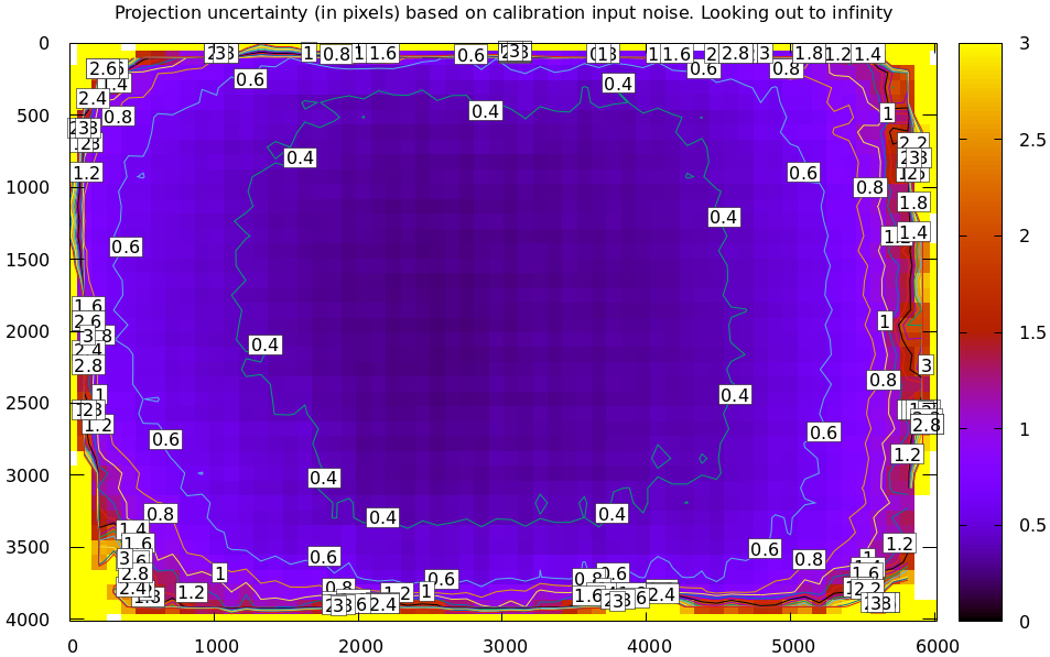
As expected, the splined model doesn't have the stiffness of LENSMODEL_OPENCV8, so we get
the less optimistic (but more realistic) uncertainty reports.
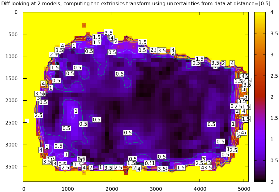
The effect of range in differencing and uncertainty computations
Earlier I talked about model differencing and estimation of projection uncertainty. In both cases I glossed over one important detail that I would like to revisit now. A refresher:
- To compute a diff, I unproject \(\vec q_0\) to a point in space \(\vec p\) (in camera coordinates), transform it, and project that back to the other camera to get \(\vec q_1\)
- To compute an uncertainty, I unproject \(\vec q_0\) to (eventually) a point in space \(\vec p_\mathrm{fixed}\) (in some fixed coordinate system), then project it back, propagating all the uncertanties of all the quantities used to compute the transformations and projection.
The significant part is the specifics of "unproject \(\vec q_0\)". Unlike a projection operation, an unprojection is ambiguous: given some camera-coordinate-system point \(\vec p\) that projects to a pixel \(\vec q\), we have \(\vec q = \mathrm{project}\left(k \vec v\right)\) for all \(k\). So an unprojection gives you a direction, but no range. What that means in this case, is that we must choose a range of interest when computing diffs or uncertainties. It only makes sense to talk about a "diff when looking at points \(r\) meters away" or "the projection uncertainty when looking out to \(r\) meters".
A surprising consequence of this is that while projection is invariant to scaling (\(k \vec v\) projects to the same \(\vec q\) for any \(k\)), the uncertainty of this projection is not:
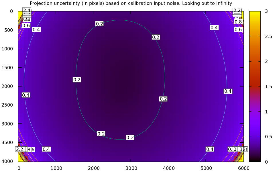
Let's look at the projection uncertainty at the center of the imager at
different ranges for the LENSMODEL_OPENCV8 model we computed earlier:
mrcal-show-projection-uncertainty --vs-distance-at center \
                                  opencv8.cameramodel --set 'yrange [0:0.3]'
So the uncertainty grows without bound as we approach the camera. As we move away, there's a sweet spot where we have maximum confidence. And as we move further out still, we approach some uncertainty asymptote at infinity. Qualitatively this is the figure I see 100% of the time, with the position of the minimum and of the asymptote varying.
Why is the uncertainty unbounded as we approach the camera? Because we're looking at the projection of a fixed point into a camera whose position is uncertain. As we get closer to the origin of the camera, the noise in the camera position dominates the projection, and the uncertainty shoots to infinity.
What controls the range where we see the lowest uncertainty? The range where we observed the chessboards. I will prove this conclusively in the next section. It makes sense: the lowest uncertainty corresponds to the region where we have the most information.
What controls the uncertainty at infinity? I don't have an intuitive answer, but we'll get a good sense from experiments in the next section.
This is a very important effect to characterize. In many applications the range of observations at calibration time will vary significantly from the working range post-calibration. For instance, any application involving wide lenses will use closeup calibration images, but working images from further out. We don't want to compute a calibration where the calibration-time uncertainty is wonderful, but the working-range uncertainty is poor.
I should emphasize that while unintuitive, this uncertainty-depends-on-range effect is very real. It isn't just something that you get out of some opaque equations, but it's observable in the field. Here're two real-world diffs of two calibrations computed from different observations made by the same camera a few minutes apart. Everything is the same, so I should be getting identical calibrations. A diff at infinity:
mrcal-show-projection-diff --unset key camera[01].cameramodel
And again at 0.5m (close to the range to the chessboards)
mrcal-show-projection-diff --distance 0.5 --unset key camera[01].cameramodel
Clearly the prediction that uncertainties are lowest at the chessboard range, and rise at infinity is borne out here by just looking at diffs, without computing the uncertainty curves. I didn't have to look very hard to find calibrations that showed this. Any calibration from suboptimal chessboard images (see next section) shows this effect. I didn't use the calibrations from this document because they're too good to see this clearly.
Optimal choreography
Now that we know how to measure calibration quality and what to look for, we can
run some studies to figure out what makes a good chessboard dance. These are all
computed by the analyses/dancing/dance-study.py tool. It generates synthetic
data, scans a parameter, and produces the uncertainty-vs-range curves at the
imager center to visualize the effect of that parameter.
I run all of these studies using the LENSMODEL_OPENCV8 model computed above. It computes
faster than the splined model, and qualitatively produces the similar results.
How many chessboard observations should we get?
dance-study.py --scan Nframes --Ncameras 1 --Nframes 20,200 --range 0.5 \
               --observed-pixel-uncertainty 2 --ymax 1 \
               opencv8.cameramodel
Here I'm running a monocular solve that looks at chessboards ~ 0.5m away, scanning the frame count from 20 to 200.
The horizontal dashed line is the uncertainty of the input noise observations. Looks like we can usually do much better than that. The vertical dashed line is the mean distance where we observed the chessboards. Looks like the sweet spot is a bit past that.
And it looks like more observations is always better, but we reach the point of diminishing returns at ~ 100 frames.
OK. How close should the chessboards be?
dance-study.py --scan range --Ncameras 1 --Nframes 100 --range 0.4,10 \
               --observed-pixel-uncertainty 2 \
               opencv8.cameramodel
This effect is dramatic: we want closeups. Anything else is a waste of time. Here we have two vertical dashed lines, indicating the minimum and maximum ranges I'm scanning. And we can see, the the sweet spot for each trial moves further back as we move the chessboards back.
Alrighty. Should the chessboards be shown head-on, or should they be tilted?
dance-study.py --scan tilt_radius --tilt-radius 0,80 --Ncameras 1 --Nframes 100 \
               --range 0.5 \
               --observed-pixel-uncertainty 2 --ymax 2 --uncertainty-at-range-sampled-max 5 \
               opencv8.cameramodel
The head-on views (tilt = 0) produce quite poor results. And we get more and more confidence with more board tilt, with diminishing returns at about 45 degrees.
We now know that we want closeups and we want tilted views. This makes intuitive sense: a tilted close-up view is the best-possible view to tell the solver whether the size of the observed chessboard is caused by the focal length of the lens or by the distance of the observation to the camera. The worst-possible observations for this are head-on far-away views. Given such observations, moving the board forward/backward and changing the focal length have a very similar effect on the observed pixels.
Also this clearly tells us that chessboards are the way to go, and a calibration object that contains a grid of circles will work badly. Circle grids work either by finding the centroid of each circle "blob" or by fitting a curve to the circle edge to infer the location of the center. A circle viewed from a tilted closeup will appear lopsided, so we have a choice of suffering a bias from imprecise circle detections or getting poor uncertainties from insufficient tilt. Extra effort can be expended to improve this situation, or chessboards can be used.
And let's do one more. Often we want to calibrate multiple cameras, and we are free to do one N-way calibration or N separate monocular calibrations or anything in-between. The former has more constraints, so presumably that would produce less uncertainty. How much?
I'm processing the same calibration geometry, varying the number of cameras from 1 to 8. The cameras are all in the same physical location, so they're all seeing the same thing (modulo the noise), but the solves have different numbers of parameters and constraints.
dance-study.py --scan Ncameras --Ncameras 1,8 --camera-spacing 0 --Nframes 100 \
               --range 0.5 --ymax 0.4 --uncertainty-at-range-sampled-max 10 \
               --observed-pixel-uncertainty 2 \
               opencv8.cameramodel
So clearly there's a benefit to more cameras. After about 4, we hit diminishing returns.
That's great. We now know how to dance given a particular chessboard. But what kind of chessboard do we want? We can study that too.
mrcal assumes a chessboard being a planar grid. But how many points do we want in this grid? And what should the grid spacing be?
First, the point counts. We expect that adding more points to a chessboard of the same size would produce better results, since we would have strictly more data to work with. This expectation is correct:
dance-study.py --scan object_width_n --range 2 --Ncameras 1 --Nframes 100 \
               --object-width-n 5,30 \
               --uncertainty-at-range-sampled-max 30 \
               --observed-pixel-uncertainty 2 \
               opencv8.cameramodel
Here we varied object-width-n, but also adjusted object-spacing to keep the
chessboard size the same.
What if we leave the point counts alone, but vary the spacing? As we increase the point spacing, the board grows in size, spanning more and more of the imager. We expect that this would improve the things:
dance-study.py --scan object_spacing --range 2 --Ncameras 1 --Nframes 100 \
               --object-spacing 0.04,0.20 \
               --observed-pixel-uncertainty 2 \
               opencv8.cameramodel
And they do. At the same range, a bigger chessboard is better.
Finally, what if we increase the spacing (and thus the board size), but also move the board back to compensate, so the apparent size of the chessboard stays the same? I.e. do we want a giant board faraway, or a tiny board really close in?
dance-study.py --scan object_spacing --range 2 --Ncameras 1 --Nframes 100 \
               --object-spacing 0.04,0.20 \
               --observed-pixel-uncertainty 2 --scan-object-spacing-compensate-range \
               --ymax 20 --uncertainty-at-range-sampled-max 200 \
               opencv8.cameramodel
Looks like the optimal uncertainty is the same in all cases, but tracks the moving range. The uncertainty at infinity is better for smaller boards closer to the camera. This is expected: tilted closeups span a bigger set of relative ranges to the camera.
Conclusions:
- More frames are good
- Closeups are extremely important
- Tilted views are good
- A smaller number of bigger calibration problems is good
- More chessboard corners is good, as long as the detector can find them reliably
- Tiny chessboards near the camera are better than giant far-off chessboards. As long as the camera can keep the chessboards and the working objects in focus
None of these are surprising, but it's good to see the effects directly from the data. And we now know exactly how much value we get out of each additional observation or an extra little bit of board tilt or some extra chessboard corners.
Before moving on, I should say that these are very conclusive results qualitatively. But specific recommendations about how to dance and what kind of board to use vary, depending on the specific kind of lens and geometry. Rerun these studies for your use cases, if conclusive results are needed.
Stereo
Finally, let's do some stereo processing. Originally mrcal wasn't intended to do this, but its generic capabilities in manipulating images, observations, geometry and lens models made core stereo functionality straightforward to implement. So when I hit some problems with existing tools, I added these functions to mrcal.
Formulation
What does "stereo processing" mean? I do usual epipolar geometry thing:
- Ingest two camera models, each containing the intrinsics and the relative pose between the two cameras
- And a pair of images captured by these two cameras
- Transform the images to construct "rectified" images
- Perform "stereo matching". For each pixel in the left rectified image we try to find the corresponding pixel in the same row of the right rectified image. The difference in columns is written to a "disparity" image. This is the most computationally-intensive part of the process
- Convert the "disparity" image to a "range" image using some basic geometry
The usual stereo matching routines have a hard requirement: all pixels
- in any given row in the left rectified image and
- in the same row in the right rectified image
contain observations from the same plane in space. This allows for one-dimensional stereo-matching, which is a massive computational win over the two-dimensional matching that would be required with another formulation. We thus transform our images into the space of \(\phi\) (the "elevation"; the tilt of the epipolar plane) and \(\theta\) (the "azimuth"; the lateral angle inside the plane):
Let's do it!
We computed intrinsics from chessboards observations earlier, so let's use these for stereo processing. I only use the splined model here.
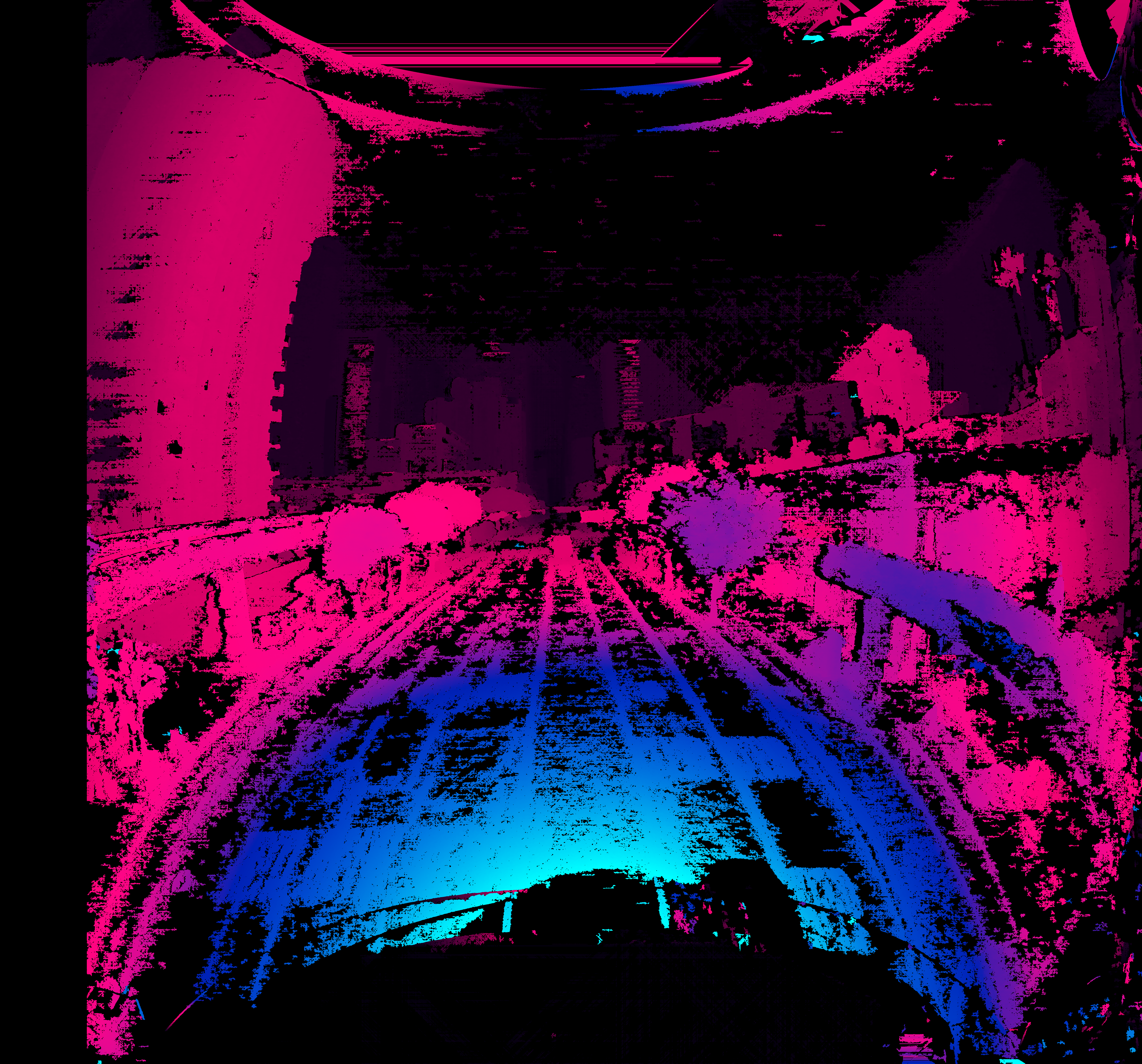
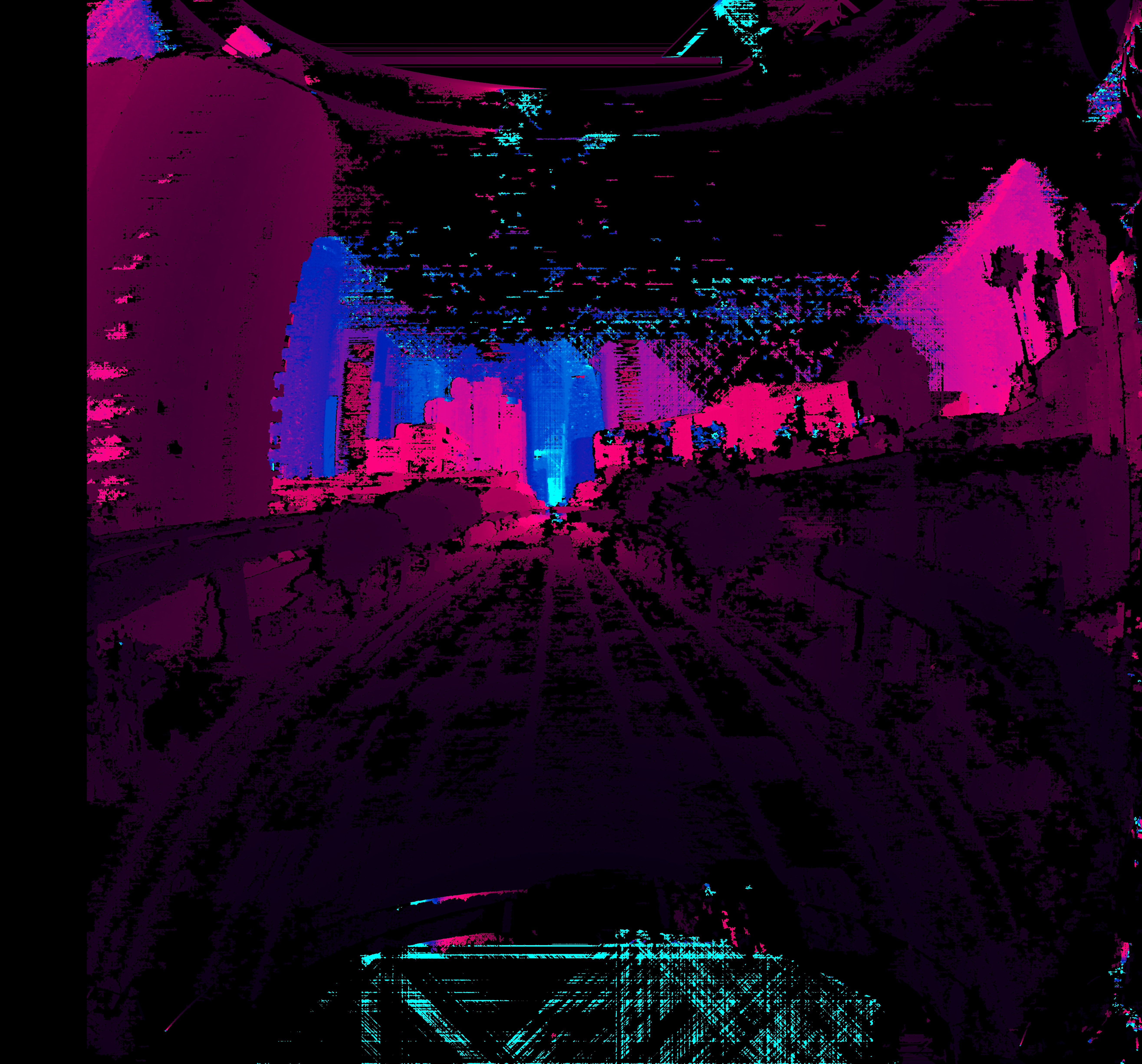
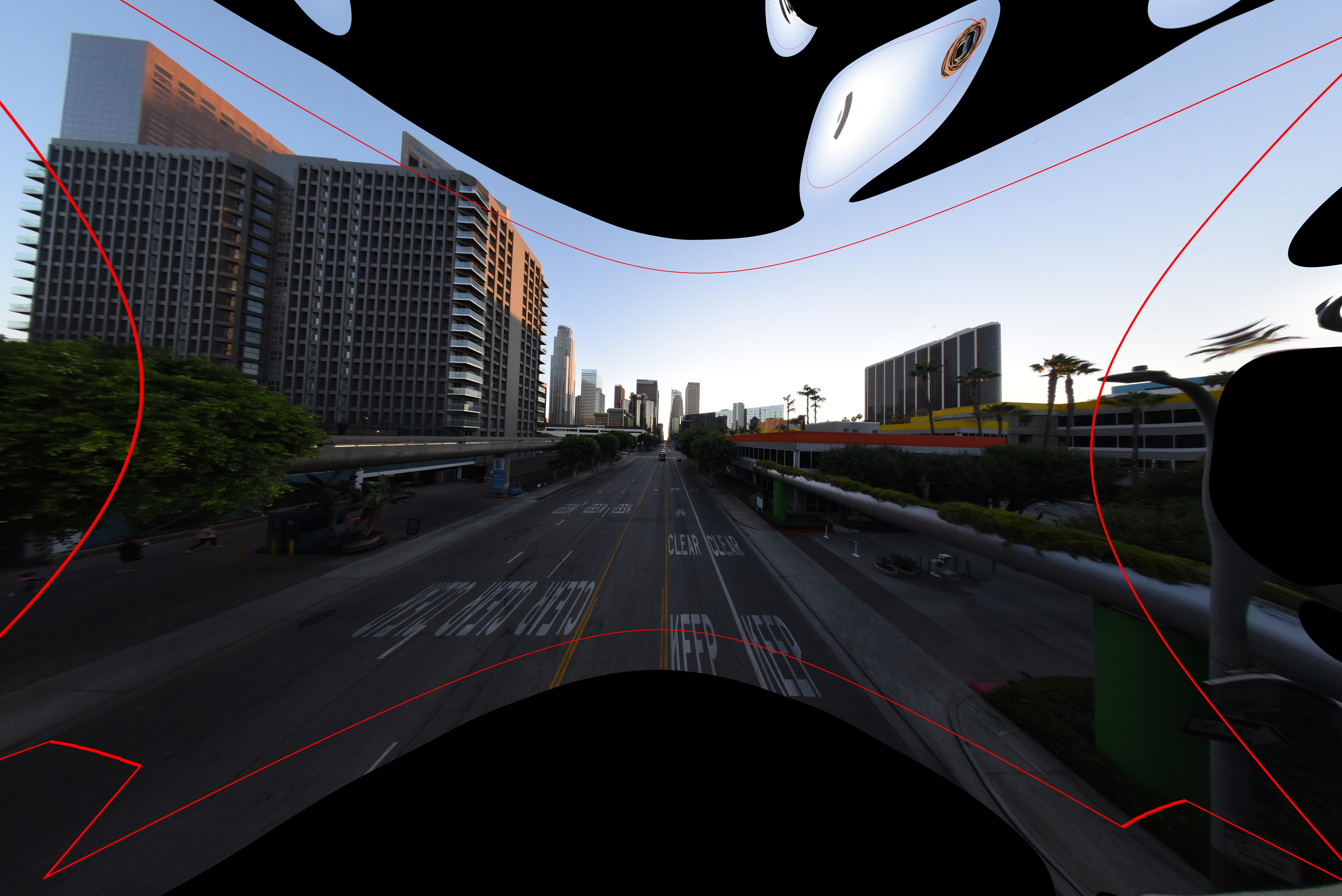
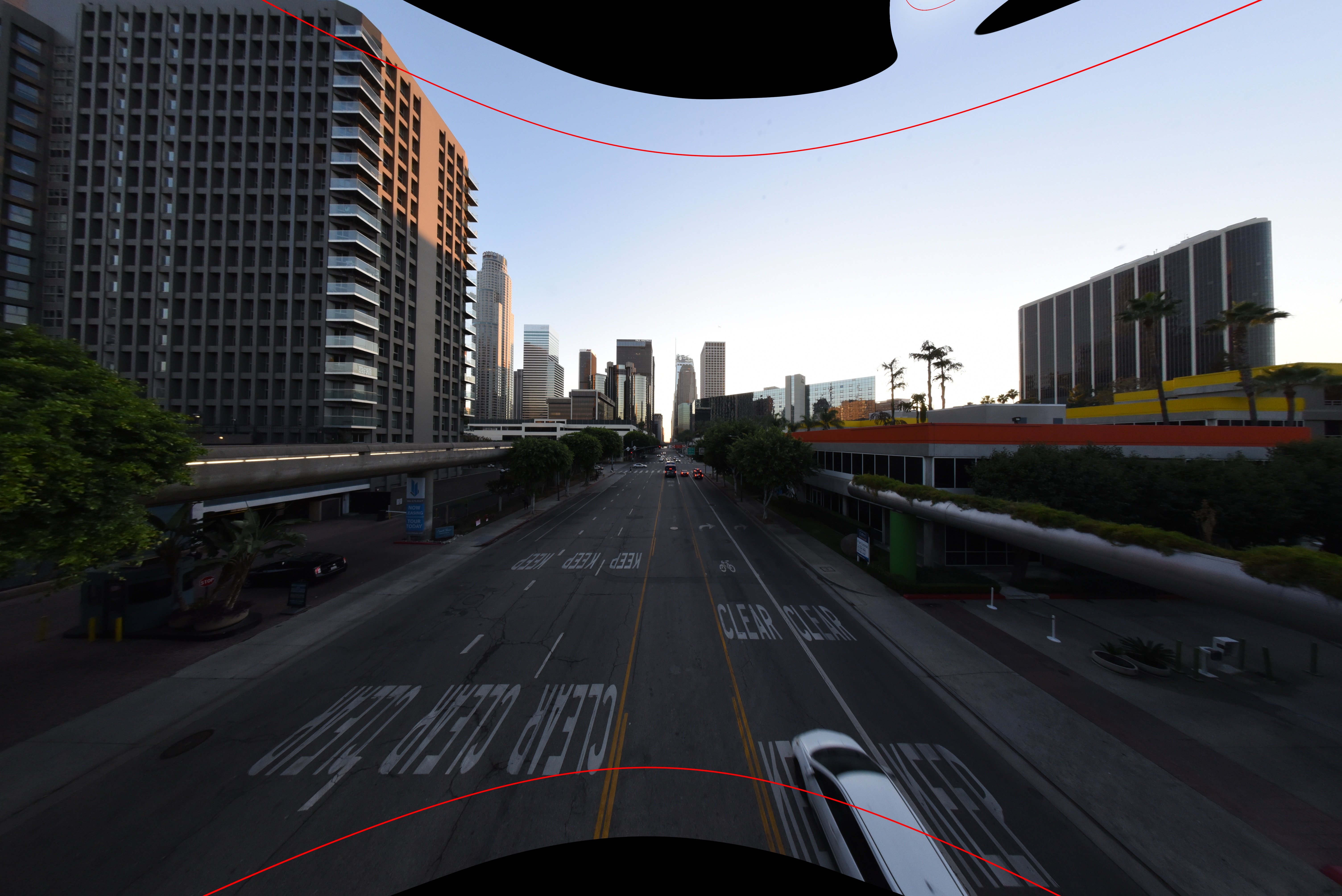
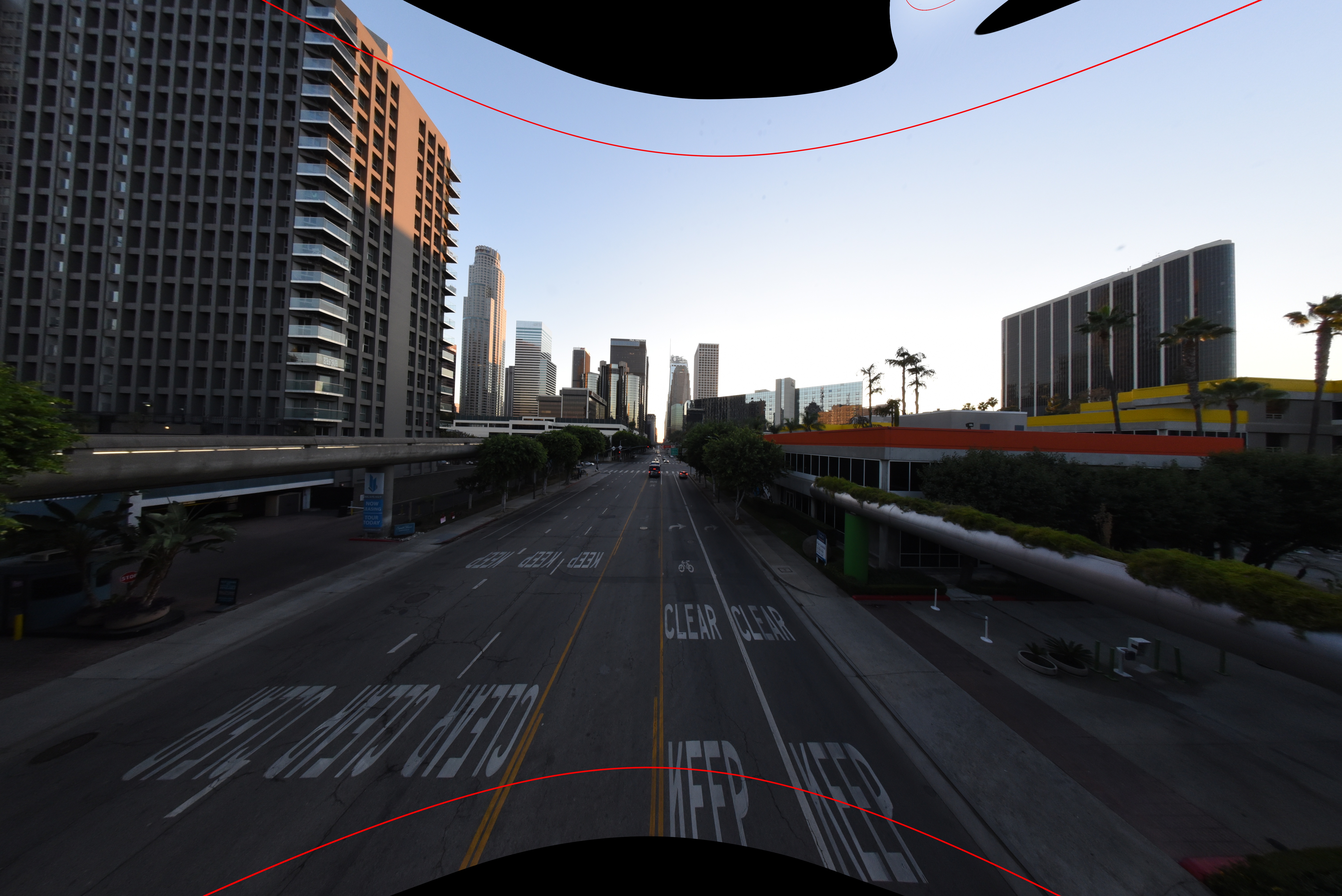
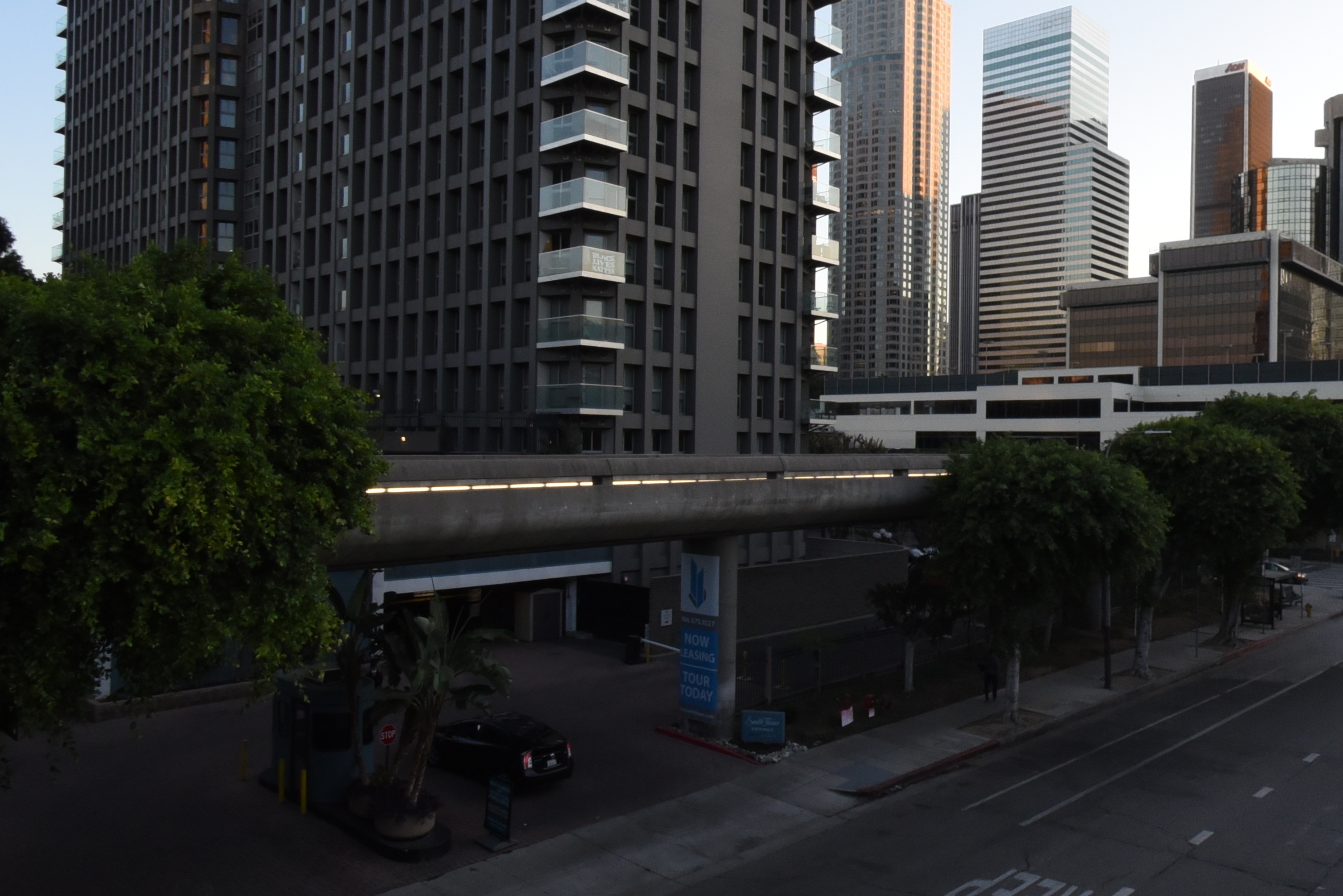
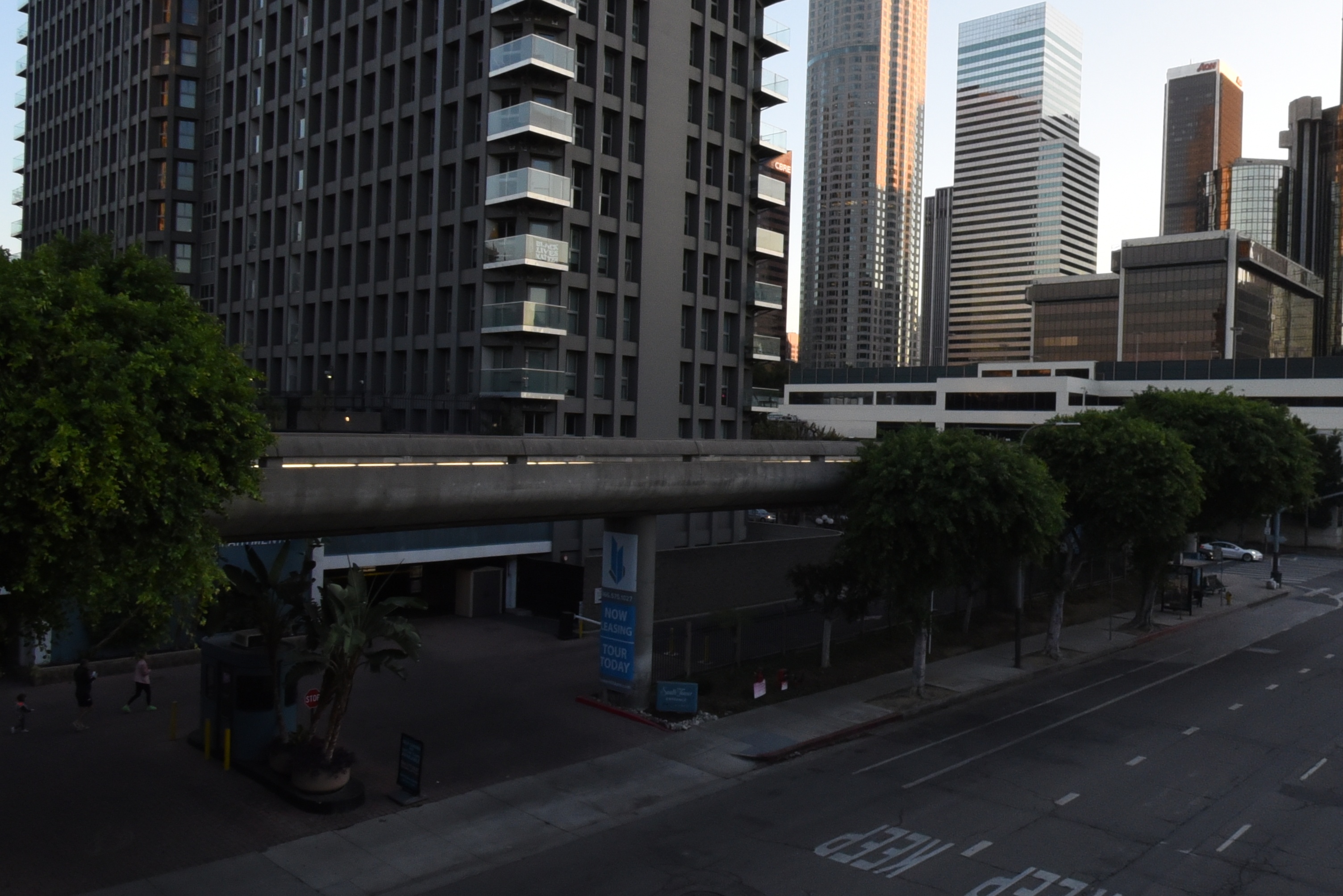
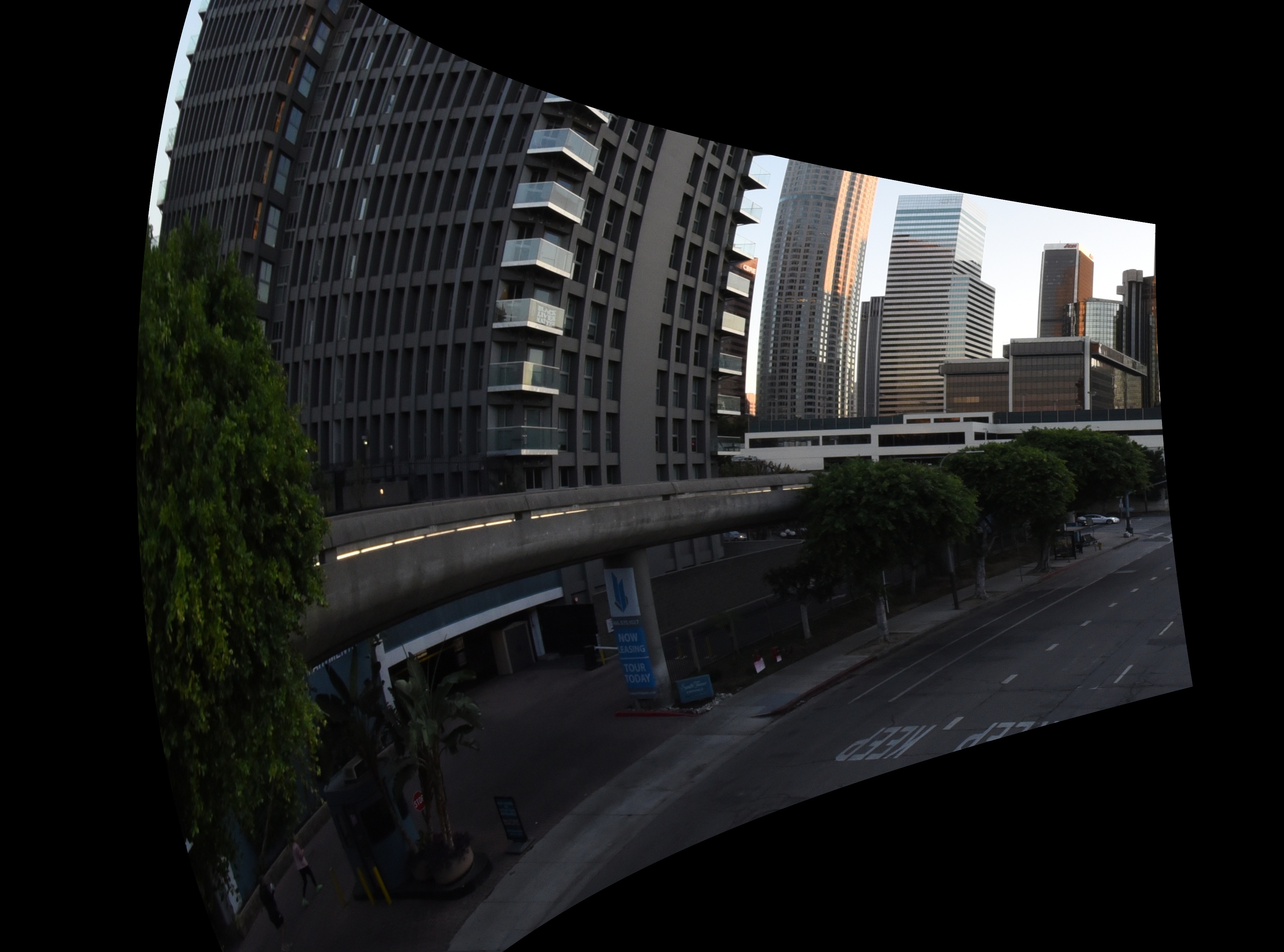
I took several images off a catwalk over Figueroa St in downtown Los Angeles. This is the view S along Figueroa St. There're tall buildings ahead and on either side, making for an interesting stereo scene.
The two images out of the camera look like this:
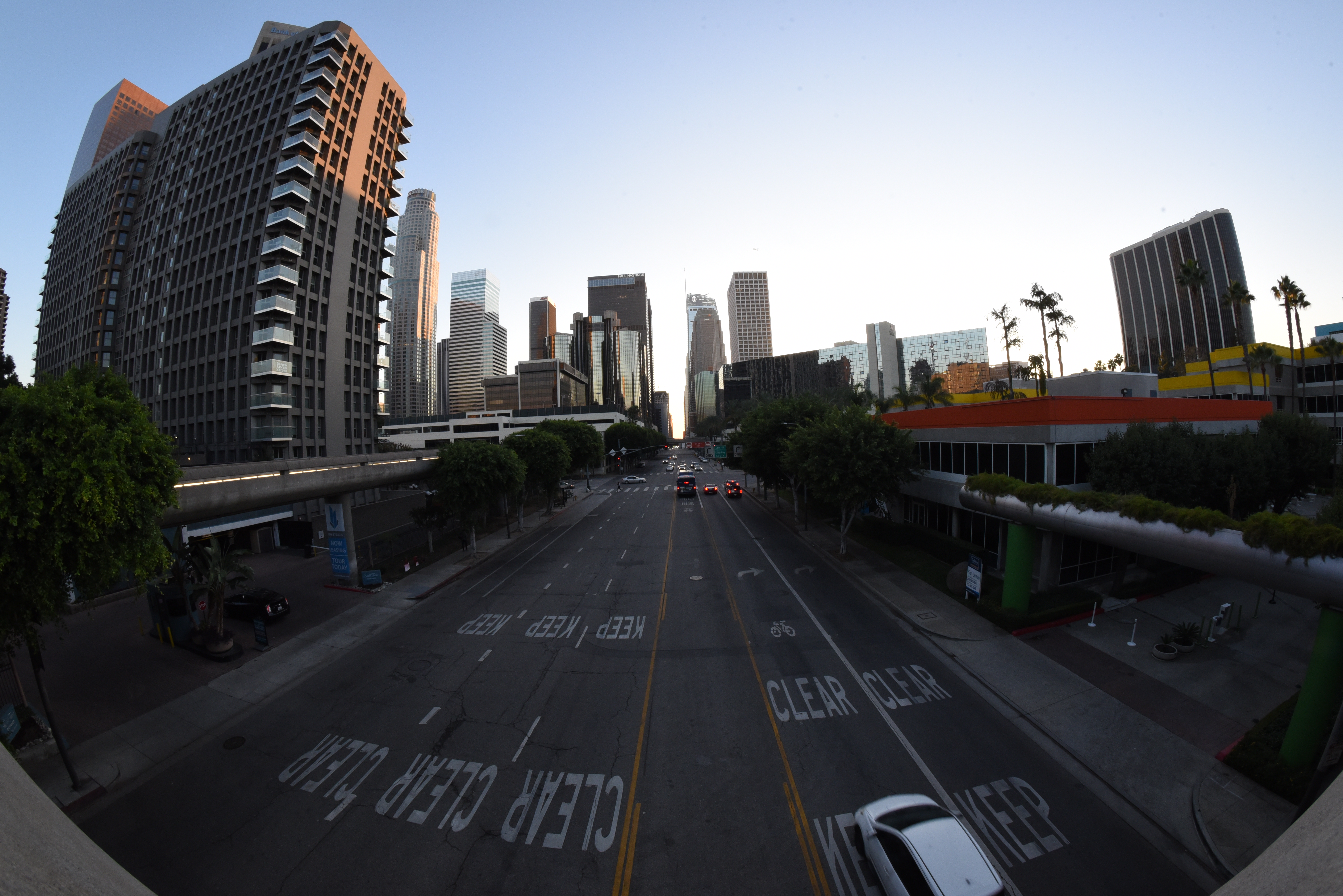
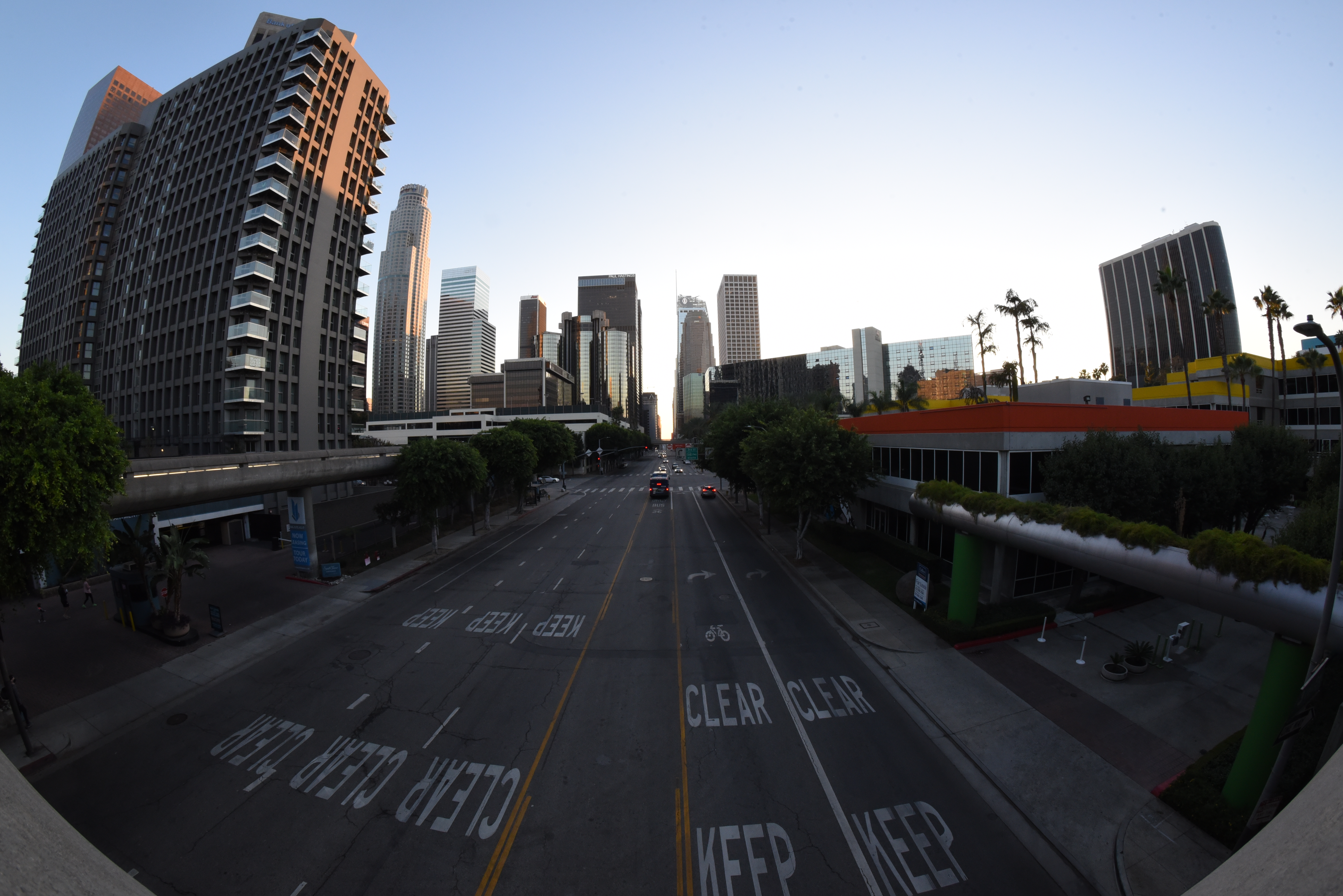
All the full-size images are available by clicking on an image.
The cameras are 7ft (2.1m) apart. In order to compute stereo images we need an accurate estimate of the geometry of the cameras. Usually we get this as an output of the calibration, but here I only had one camera to calibrate, so I don't have this geometry estimate. I used a separate tool to compute the geometry from corresponding feature detections. The details aren't important; for the purposes of this document we can assume that we did calibrate a stereo pair, and that's where the geometry came from. The resulting with-geometry models:
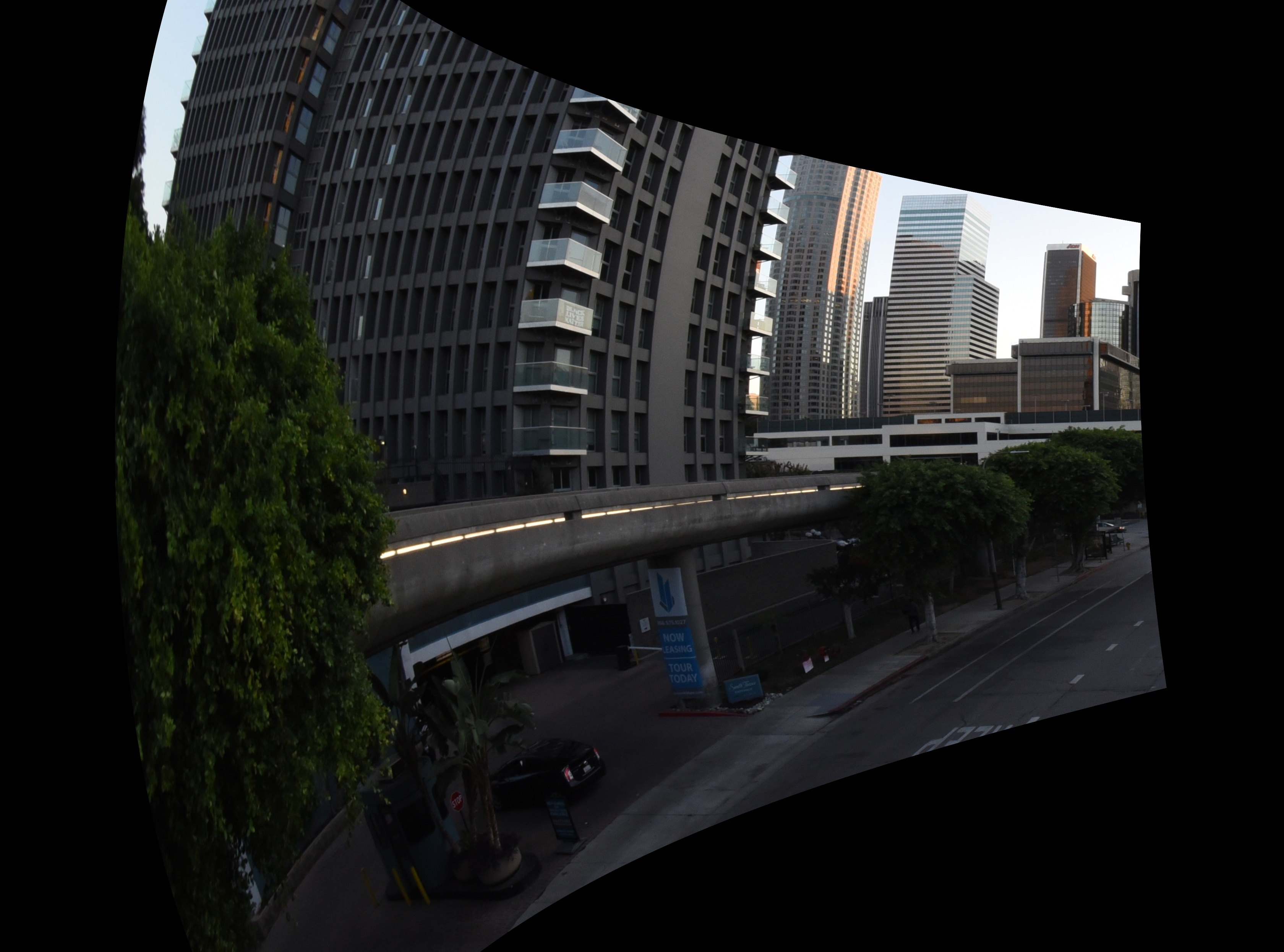
I then use the mrcal APIs to compute rectification maps, rectify the images,
compute disparities and convert them to ranges. This is done with the script
stereo.py. We run it like this:
python3 stereo.py splined-[01].cameramodel [01].jpg splined
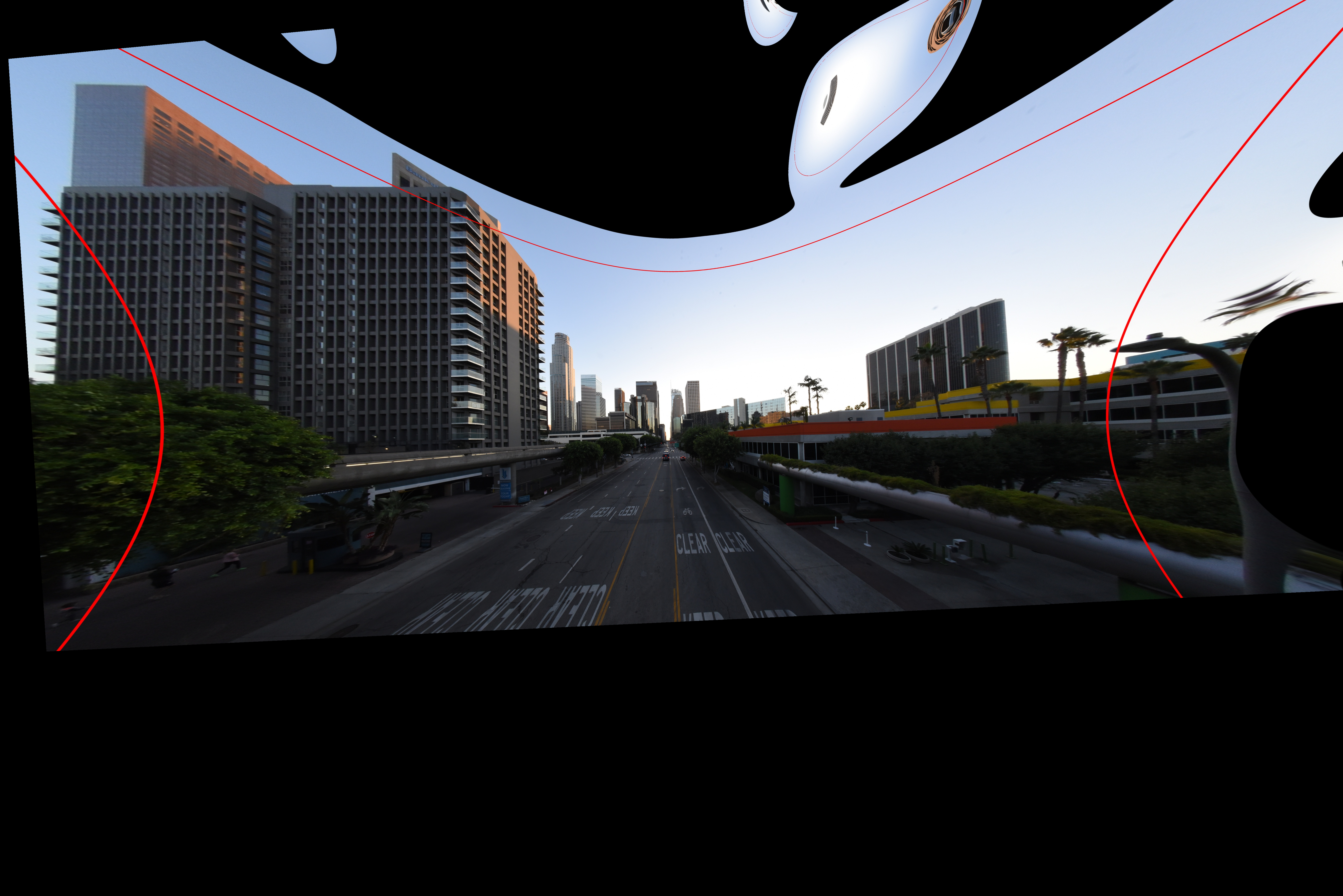
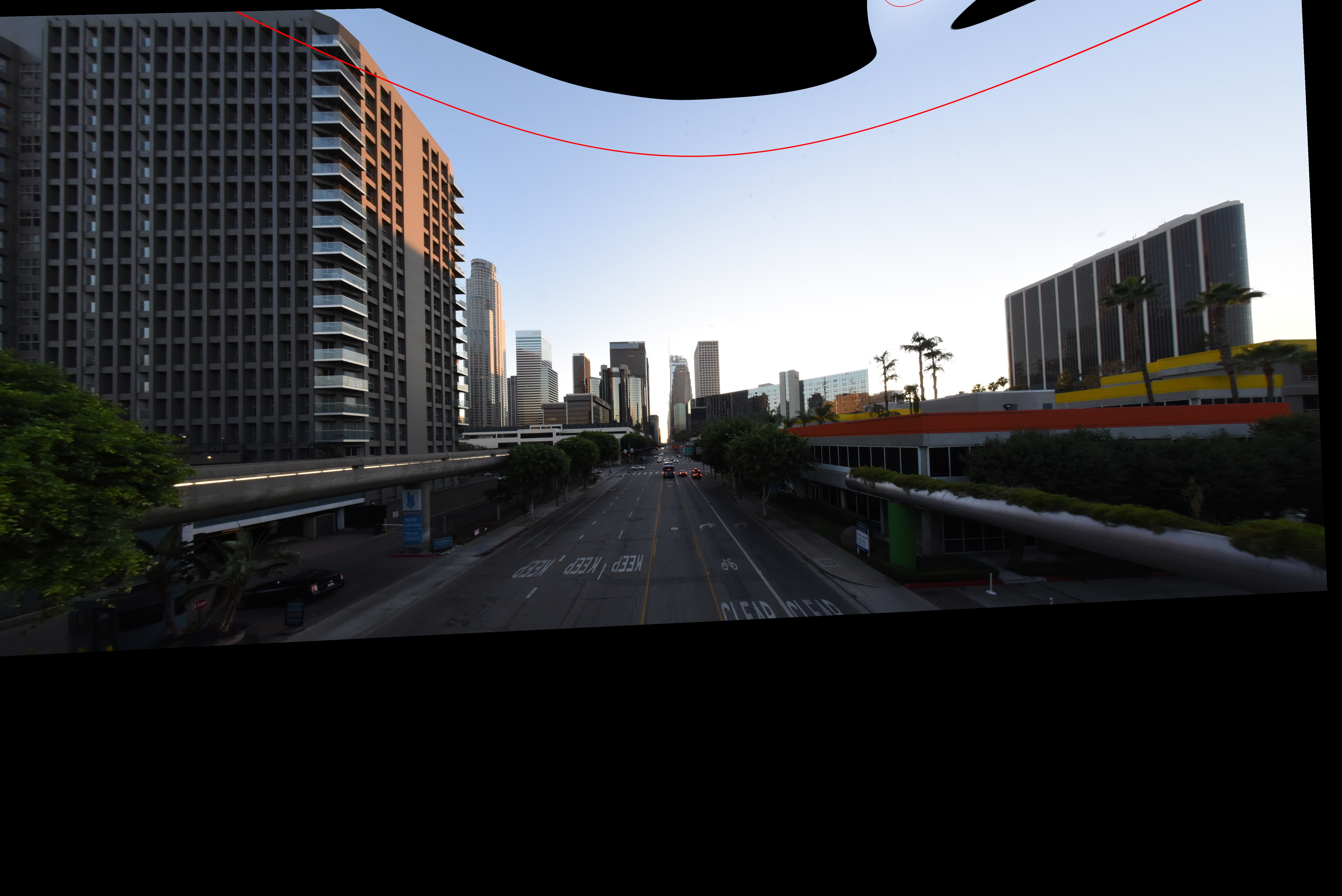
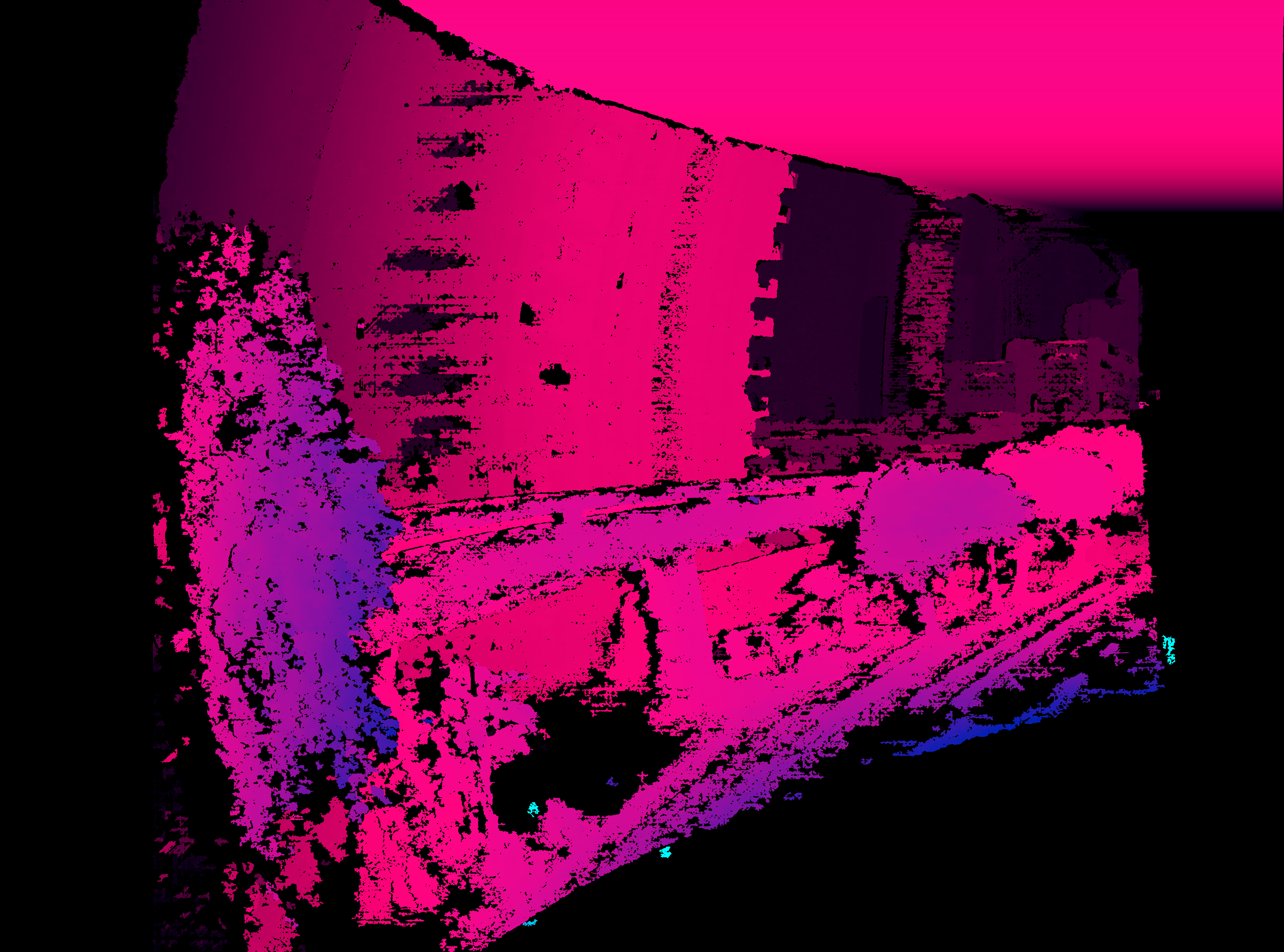
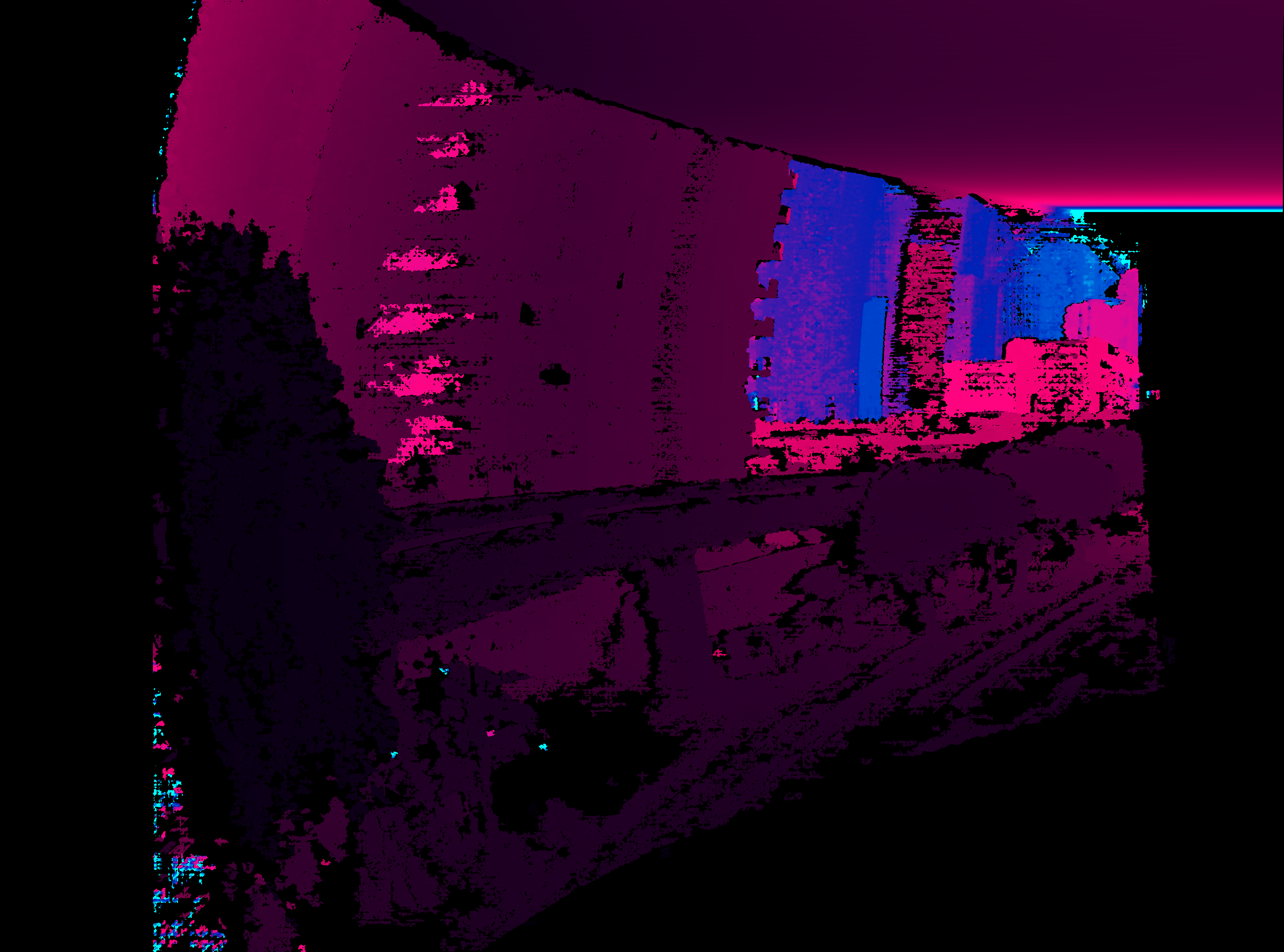
The rectified images look like this:

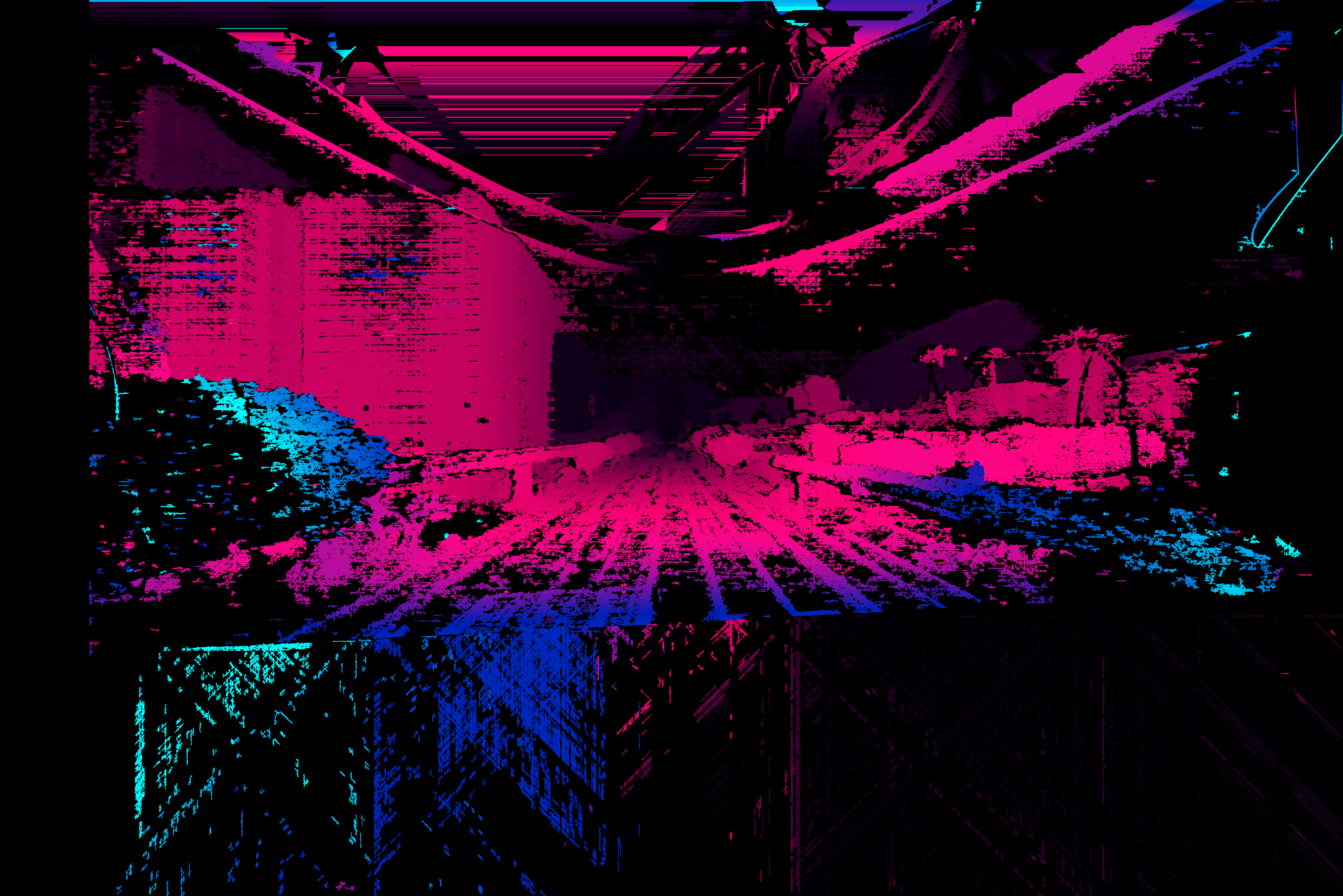
And the disparity and range images looks like this:
Clearly this is working well.
If you've used other stereo libraries previously, these rectified images may look odd. In mrcal I produce images that sample the azimuth and elevation angles evenly, which should minimize visual distortion inside each image row. A side-effect is the the vertical expansion in the rectified image at the azimuth extremes. Stereo matching works primarily by correlating the rows independently, so this is a good trade-off. Some other implementations use un-even azimuth spacing, which can't be good for matching performance.
Stereo rectification outside of mrcal
What if we want to do our stereo processing with some other tool, and what if that tool doesn't support the splined model we want to use? We can use mrcal to reproject the image to whatever model we like, and then hand off the processed image and new models to that tool. Let's demonstrate with a pinhole model.
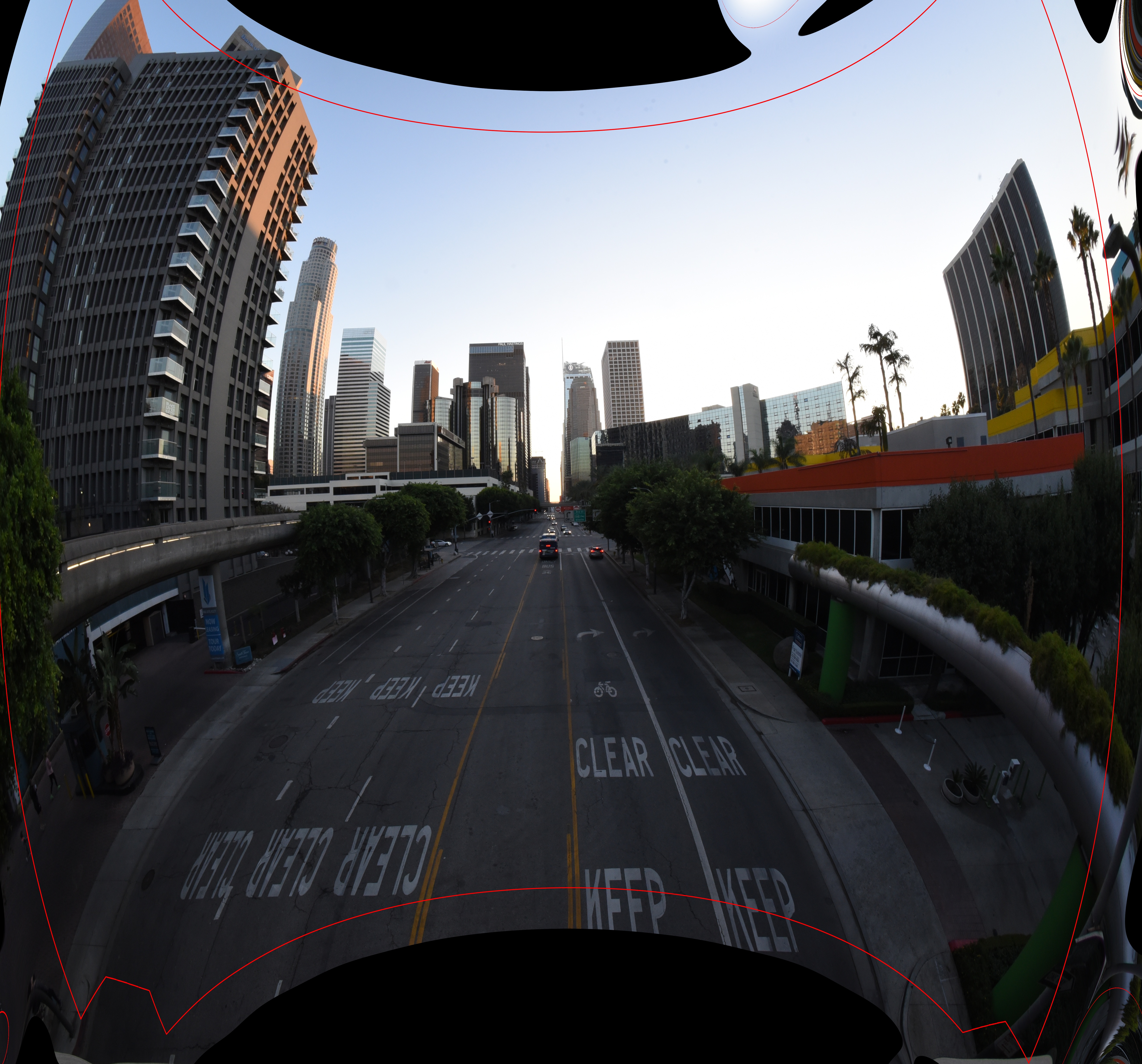
We can use the mrcal-reproject-image tool to reproject the images. Mapping
fisheye images to a pinhole model introduces an unwinnable trade-off: the
angular resolution changes dramatically as you move towards the edges of the
image. At the edges the angular resolution becomes tiny, and you need far more
pixels to represent the same arc in space as you do in the center. So you
usually need to throw out pixels in the center, and gain low-information pixels
at the edges (the original image doesn't have more resolutions at the edges, so
we must interpolate). Cutting off the edges (i.e. using a narrower lens) helps
bring this back into balance.
So let's do this using two different focal lengths:
--scale-focal 0.35: fairly wide. Looks extreme in a pinhole projection--scale-focal 0.6: not as wide. Looks more reasonable in a pinhole projection, but we cut off big chunks of the image at the edges
for scale in 0.35 0.6; do
  for c in 0 1; do
    mrcal-reproject-image       \
      --valid-intrinsics-region \
      --to-pinhole              \
      --scale-focal $scale      \
      splined-$c.cameramodel    \
      $c.jpg                    \
    | mrcal-to-cahvor           \
    > splined-$c.scale$scale.cahvor;

    mv $c-reprojected{,-scale$scale}.jpg;
  done
done
We will use jplv (a stereo library used at NASA/JPL) to process these pinhole
images into a stereo map, so I converted the models to the .cahvor file
format, as that tool expects.
The wider pinhole resampling of the two images:

The narrower resampling of the two images:
And the camera models:
- camera 0, wider scaling
- camera 1, wider scaling
- camera 0, narrower scaling
- camera 1, narrower scaling
Both clearly show the uneven resolution described above, with the wider image being far more extreme. I can now use these images to compute stereo with jplv:
for scale in 0.35 0.6; do \
  stereo --no-ran --no-disp --no-pre --corr-width 5 --corr-height 5 \
         --blob-area 10 --disp-min 0 --disp-max 400                 \
         splined-[01].scale$scale.cahvor                            \
         [01]-reprojected-scale$scale.jpg;

  for f in rect-left rect-right diag-left; do \
    mv 00-$f.png jplv-stereo-$f-scale$scale.png;
  done
done
The rectified images look like this.
For the wider mapping:

For the narrow mapping:

Here we see that jplv's rectification function also has some implicit pinhole projection assumption in there, and the scale within each row is dramatically uneven.
The above command gave me jplv's computed disparities, but to compare apples-to-apples, let's re-compute them using the same opencv routine from above:
python3 stereo.py - - jplv-stereo-rect-{left,right}-scale0.35.png jplv-scale0.35
python3 stereo.py - - jplv-stereo-rect-{left,right}-scale0.6.png  jplv-scale0.6
Looks reasonable.
Splitting a wide view into multiple narrow views
So we can use jplv to handle mrcal lenses in this way, but at the cost of degraded feature-matching accuracy due to unevenly-scaled rectified images. A way to resolve the geometric challenges of wide-angle lenses would be to subdivide the wide field of view into multiple narrower virtual lenses. Then we'd have several narrow-angle stereo pairs instead of a single wide stereo pair.
mrcal makes necessary transformations simple, so let's do it. For each image we need to construct
- The narrow pinhole model we want that looks at the area we want to (45 degrees to the left in this example)
- The image of the scene that such a model would have observed
This requires writing a little bit of code: narrow-section.py. Let's run that
for each of my images:
python3 narrow-section.py splined-0.cameramodel 0.jpg -45 left
python3 narrow-section.py splined-1.cameramodel 1.jpg -45 right
The images look like this:
Note that these are pinhole images, but the field of view is much more narrow, so they don't look distorted like before. The corresponding pinhole models:
We can feed these to the stereo.py tool as before:
python3 stereo.py                               \
  pinhole-narrow-yawed-{left,right}.cameramodel \
  narrow-{left,right}.jpg                       \
  narrow
Here we have slightly non-trivial geometry, so it is instructive to visualize it
(the stereo.py tool does this):
Here we're looking at the left and right cameras in the stereo pair, and at
the axes of the stereo system. Now that we have rotated each camera to look to
the left, the baseline is no longer perpendicular to the central axis of each
camera. The stereo system is still attached to the baseline, however. That means
that \(\theta = 0\) no longer corresponds to the center of the view. We don't need
to care, however: mrcal.stereo_rectify_prepare() figures that out, and
compensates.
And we get nice-looking rectified images:
And disparity and range images:
And this is despite running pinhole-reprojected stereo from a very wide lens.