How to run a calibration

We need to get observations of a calibration object, a board containing an observable grid of points. mrcal doesn't care where these observations come from, but the recommended method is to use a chessboard target, and to employ the mrgingham detector. The mrgingham documentation has a .pdf of a chessboard pattern that works well. This pattern should be printed and mounted onto a rigid and flat surface to produce the calibration object. According to the dance study, we want the chessboard to be as small as possible, to allow close-up views of the board that fill the imager. The limiting factor is the camera's depth of field: we want both the calibration-time close-up views and the working-range images to be in focus at the same time. If a too-small board is used, the imager-filling close-ups will be out of focus.

Calibrating wide lenses generally requires large chessboards: I use a square chessboard roughly 1m per side to calibrate my fisheye lenses. A big chessboard such as this is never completely rigid or completely flat, so my board is backed with 2cm of foam. This keeps the shape stable over short periods of time, which is sufficient for our purposes. mrcal estimates the chessboard shape as part of its calibration solve, so a non-planar deformation is acceptable, as long it is stable over the course of a board dance.

Now that we have a calibration object, this object needs to be shown to the camera(s). It is important that the images contain clear features. Motion blur or focus or exposure issues will all cause bias in the resulting calibration.

If calibrating multiple cameras, mrcal will solve for all the intrinsics and extrinsics. There is one strong requirement on the captured images in this case: the images must be synchronized across all the cameras. This allows mrcal to assume that if camera A and camera B observed a chessboard at time T, then this chessboard was at exactly the same location when the two cameras saw it. Generally this means that either

• The cameras are wired to respond to a physical trigger signal
• The chessboard and cameras were physically fixed (on a tripod, say) at each time of capture

Some capture systems have a "software" trigger mode, but this is usually too loose to produce usable results. A similar consideration exists when using cameras with a rolling shutter. With such cameras it is imperative that everything remain stationary during image capture, even when only one camera is involved.

If synchronization or rolling shutter effects are in doubt, look at the residual plot made by show_residuals_observation_worst() (a sample and a description appear below). These errors clearly show up as distinct patterns in those plots.

As shown in the dance study, the most useful observations to gather are

• close-ups: the chessboard should fill the whole frame as much as possible. Small chessboards next to the camera are preferred to larger chessboards further out; the limit is set by the depth of field.
• oblique views: tilt the board forward/back and left/right. I generally tilt by ~ 45 degrees. At a certain point the corners become indistinct and mrgingham starts having trouble, but depending on the lens, that point could come with quite a bit of tilt. A less dense chessboard eases this also, at the cost of requiring more board observations to get the same number of points.
• If calibrating multiple cameras, it is impossible to place a calibration object at a location where it's seen by all the cameras and where it's a close-up for all the cameras. So you should get close-ups for each camera individually, and also get observations common to multiple cameras, that aren't necessarily close-ups. The former will serve to define your camera intrinsics, and the latter will serve to define your extrinsics (geometry). Get just far-enough out to create the joint views. If usable joint views are missing, the extrinsics will be undefined, and the solver will complain about a "not positive definite" (singular in this case) Hessian.

A dataset composed primarily of tilted closeups produces good results.

If the model will be used to look at far-away objects, care must be taken to produce a reliable calibration at long ranges, not just at the short ranges where the chessboards were. Close-up chessboard views are the primary data needed to get good uncertainties at infinity, but quite often these will produce images that aren't in focus (if the focus ring is set to the working range: infinity). See the dance study for detail. Cameras meant for outdoor stereo and/or wide lenses usually have this problem. In such cases, it is strongly recommended to re-run the dance study for your particular use case to get a sense of what kind of observations are required, and what kind of uncertainties can be expected. The current thought is that the best thing to do is to get close-up images even if they're out of focus. The blurry images will have a high --observed-pixel-uncertainty (and no bias; hopefully), but the uncertainty reduction you get from the close-ups more than makes up for it. In these cases you usually need to get more observations than you normally would to bring down the uncertainties to an acceptable level.

It is better to have more data rather than less. mrgingham will throw away frames where no chessboard can be found, so it is perfectly reasonable to grab too many images with the expectation that they won't all end up being used in the computation.

I usually aim for about 100 usable frames, but you can often get away with far fewer. The mrcal uncertainty feedback (see below) will tell you if you need more data.

Naturally, intrinsics are accurate only in areas where chessboards were observed: chessboard observations on the left tell us little about lens behavior on the right. Thus it is imperative to cover the whole field of view during the chessboard dance. It is often tricky to get good data at the edges and corners of the imager, so care must be taken. Some chessboard detectors (mrgingham in particular) only report complete chessboards. This makes it extra-challenging to obtain good data at the edges: a small motion that pushes one chessboard corner barely out of bounds causes the whole observation to be discarded. It is thus very helpful to be able to see a live feed of the camera, as the images are being captured. In either case, visualizing the obtained chessboard detections is very useful to see if enough coverage was obtained.

With monocular calibrations, there're no requirements on image filenames: use whatever you like. If calibrating multiple synchronized cameras, however, the image filenames would need to indicate what camera captured each image at which time. I generally use frameFFF-cameraCCC.jpg. Images with the same FFF are assumed to have been captured at the same instant in time, and CCC identifies the camera. Naming images in this way is sufficient to communicate these mappings to mrcal.

Once mrgingham is installed or built from source, it can be run by calling the mrgingham executable. The sample in the tour of mrcal processes these images to produce these chessboard corners like this:

mrgingham -j3 '*.JPG' > corners.vnl 

mrgingham tries to handle a variety of lighting conditions, including varying illumination across the image, but the corners must exist in the image in some form. mrgingham returns only complete chessboard views: if even one corner of the chessboard couldn't be found, mrgingham will discard the entire image. Thus it takes care to get data at the edges and in the corners of the imager. Another requirement due to the design of mrgingham is that the board should be held with a flat edge parallel to the camera xz plane (parallel to the ground, usually). mrgingham looks for vertical and horizontal sequences of corners, but if the board is rotated diagonally, then none of these sequences are clearly "horizontal" or "vertical".

If we use a grid detector other than mrgingham, we need to produce a compatible corners.vnl file. This is a vnlog (text table) where each row describes a single corner detection. The whole chessboard is described by a sequence of these corner detections, listed in a consistent grid order.

This file should contain 3 or 4 columns. The first 3 columns:

• filename: the path to the chessboard image
• x, y: pixel coordinates of the detected corner

If a 4th column is present, it describes the detector's confidence in the detection of that particular corner. It may be either

• level: the decimation level of the detected corner. If the detector needed to cut down the image resolution to find this corner, we report that resolution here. Level-0 means "full-resolution", level-1 means "half-resolution", level-2 means "quarter-resolution" and so on. A level of "-" or <0 means "skip this point"; this is how incomplete board observations are specified
• weight: how strongly to weight that corner. More confident detections take stronger weights. This should be inversely proportional to the standard deviation of the detected pixel coordinates. With decimation levels we have \(\mathrm{weight} = 2^{-\mathrm{level}}\). As before, a weight of "-" or <0 means "skip this point"; this is how incomplete board observations are specified

If no 4th column is present, we assume an even weight of 1.0 for all the points.

Images where no chessboard was detected should be omitted, or represented with a single record

FILENAME - - -

Once we have a corners.vnl from some chessboard detector, we can visualize it. This is a simple vnlog table:

$ < corners.vnl head -n5

## generated with mrgingham -j3 *.JPG
# filename x y level
DSC_7374.JPG 1049.606126 1032.249784 1
DSC_7374.JPG 1322.477977 1155.491028 1
DSC_7374.JPG 1589.571471 1276.563664 1

How well did we cover the imager? Did we get the edges and corners?

$ < corners.vnl       \
  vnl-filter -p x,y | \
  feedgnuplot --domain --square --set 'xrange [0:6016]' --set 'yrange [4016:0]'

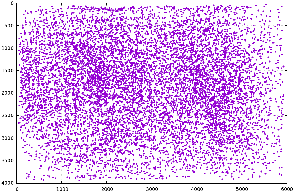
Looks like we did OK. It's a bit thin along the bottom edge, but not terrible. It is very easy to miss getting usable data at the edges, so checking this is highly recommended. If you have multiple cameras, check the coverage separately for each one. This can be done by filtering the corners.vnl to keep only the data for the camera in question. For instance, if we're looking at the left camera with images in files left-XXXXX.jpg, you can replace the above vnl-filter command with vnl-filter 'filename ~ "left"' -p x,y.

We can visualize individual detections like this:

$ f=DSC_7374.JPG

$ < corners.vnl vnl-filter "filename eq \"$f\"" --perl -p x,y,size='2**(1-level)' | \
  feedgnuplot --image $f --domain --square --tuplesizeall 3 --with 'points pt 7 ps variable'

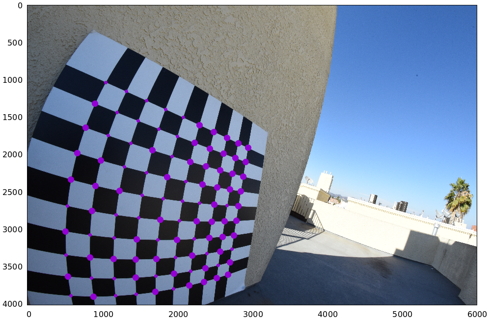
Here the size of the circle indicates the detection weight. In this image many of the corners were detected at full-resolution (level-0), but some required downsampling for the detector to find them: smaller circles. The downsampled points have less precision, so they are weighed less in the optimization. How many images produced successful corner detections?

$ < corners.vnl vnl-filter --has x -p filename | uniq | grep -v '#' | wc -l

186


$ < corners.vnl vnl-filter x=='"-"' -p filename | uniq | grep -v '#' | wc -l

89

So we have 186 images with detected corners, and 89 images where a full chessboard wasn't found. Most of the misses are probably images where the chessboard wasn't entirely in view, but some could be failures of mrgingham. In any case, 186 observations is usually plenty.

Once we have gathered our input images, we can run the calibration tool. Example, calibrating one camera at a time.

$ mrcal-calibrate-cameras        \
  --corners-cache corners.vnl    \
  --lensmodel LENSMODEL_OPENCV8  \
  --focal 1700                   \
  --object-spacing 0.077         \
  --object-width-n 10            \
  --observed-pixel-uncertainty 2 \
  --explore                      \
  '*.JPG'

• --corners-cache corners.vnl says that the chessboard corner coordinates live in a file called corners.vnl. This is the output of the corner detector. This argument may be omitted, or a non-existent file may be given. mrcal-calibrate-cameras will run mrgingham in that case, and cache the results in the given file. Thus the same command would be used to both compute the corners initially, and to reuse the pre-computed corners in subsequent runs.

  As described above, the corners.vnl file can come from any chessboard detector. If it's a detector that produces a 4th column of weights instead of a decimation level, pass in --corners-cache-has-weights

• --lensmodel specifies which lens model we're using for all the cameras. In this example we're using the LENSMODEL_OPENCV8 model. This works reasonably well for wide lenses. See the lens-model page for a description of the available models. The current recommendation is to use an opencv model (LENSMODEL_OPENCV5 for long lenses, LENSMODEL_OPENCV8 for wide lenses) initially. And once that works well, to move to the splined-stereographic model to get better accuracy and reliable uncertainty reporting. This will eventually be the model of choice for all cases, but it's still relatively new, and not yet thoroughly tested in the field. For very wide fisheye lenses, this is the only model that will work at all, so start there if you have an ultra-fisheye lens.
• --focal 1700 provides the initial estimate for the camera focal lengths, in pixels. This doesn't need to be precise, but do try to get this roughly correct if possible. The focal length value to pass to --focal (\(f_\mathrm{pixels}\)) can be derived using the stereographic model definition:

\[ f_\mathrm{pixels} = \frac{\mathrm{imager\_width\_pixels}}{4 \tan \frac{\mathrm{field\_of\_view\_horizontal}}{4}} \]

With longer lenses, the stereographic model is identical to the pinhole model. With very wide lenses, the stereographic model is the basis for the splined-stereographic model, so this expression should be a good initial estimate in all cases. Note that the manufacturer-specified "field of view" is usually poorly-defined: it's different in all directions, so use your best judgement. If only the focal length is available, keep in mind that the "focal length" of a wide lens is somewhat poorly-defined also. With a longer lens, we can assume pinhole behavior to get

\[ f_\mathrm{pixels} = f_\mathrm{mm} \frac{\mathrm{imager\_width\_pixels}}{\mathrm{imager\_width\_mm}} \]

Again, use your best judgement. This doesn't need to be exact, but getting a value in the ballpark makes life easier for the solver

• --object-spacing is the distance between neighboring corners in the chessboard
• --object-width-n is the horizontal corner count of the calibration object. In the example invocation above there is no --object-height-n, so mrcal-calibrate-cameras assumes a square 10x10 chessboard
• --observed-pixel-uncertainty 2 says that the \(x\) and \(y\) corner coordinates in corners.vnl are each distributed normally, independently, and with a standard deviation of 2.0 pixels. This is described in the noise model, and will be used for the projection uncertainty reporting. There isn't a reliable tool to estimate this currently (there's an attempt here, but it needs more testing). The recommendation is to eyeball a conservative value, and to treat the resulting reported uncertainties conservatively.
• --explore requests that after the models are computed, a REPL be opened so that the user can look at various metrics describing the output. It is recommended to use this REPL to validate the solve

After the options, mrcal-calibrate-cameras takes globs describing the images. One glob per camera is expected, and in the above example one glob was given: '*.JPG'. Thus this is a monocular solve. More cameras would imply more globs. For instance a 2-camera calibration might take arguments

'frame*-camera0.png' 'frame*-camera1.png'

Note that these are globs, not filenames. So they need to be quoted or escaped to prevent the shell from expanding it: hence '*.JPG' and not *.JPG.

When the mrcal-calibrate-cameras tool is run as given above, it spends a bit of time computing. The time needed is highly dependent on the specific problem, with richer lens models and more data and more cameras slowing it down, as expected. When finished, the tool writes the resulting models to disk, and opens a REPL for the user (since --explore was given). The final models are written to disk into camera-N.cameramodel where N is the index of the camera, starting at 0. These use the mrcal-native .cameramodel file format.

With a REPL, it's a good idea to sanity-check the solve. The tool displays a summary such as this:

RMS reprojection error: 0.8 pixels
Worst residual (by measurement): 7.2 pixels
Noutliers: 3 out of 18600 total points: 0.0% of the data
calobject_warp = [-0.00103983  0.00052493]

Wrote ./camera-0.cameramodel

Here the final RMS reprojection error is 0.8 pixels. Of the 18600 corner observations (186 observations of the board with 10*10 = 100 points each), 3 didn't fit the model well, and were thrown out as outliers. We expect the RMS reprojection error to be a bit below the true --observed-pixel-uncertainty (see below). Our estimated --observed-pixel-uncertainty was 2, so the results are reasonable, and don't raise any red flags.

High outlier counts or high reprojection errors would indicate that the model mrcal is using does not fit the data well. That would suggest some/all of these:

• Issues in the input data, such as incorrectly-detected chessboard corners, unsynchronized cameras, rolling shutter, motion blur, focus issues, etc. Keep reading for ways to get more insight
• A badly-fitting lens model. For instance LENSMODEL_OPENCV4 will not fit wide lenses. And only splined lens models will fit fisheye lenses all the way in the corners

Outlier rejection resolves these up to a point, but if at all possible, it is recommended to fix whatever is causing the issue, and then to re-run the solve.

The board flex was computed as 1.0mm horizontally, and 0.5mm vertically in the opposite direction. That is a small deflection, and sounds reasonable. A way to validate this, would be to get another set of chessboard images, to rerun the solve, and compare the new flex values to the old ones. From experience, I haven't seen the deflection values behave in unexpected ways.

So far, so good. What does the solve think about our geometry? Does it match reality? We can get a geometric plot by running a command in the REPL:

show_geometry( _set   = ('xyplane 0', 'view 80,30,1.5'),
                unset = 'key')

We could also have used the mrcal-show-geometry tool from the shell. All plots are interactive when executed from the REPL or from the shell. Here we see the axes of our camera (purple) situated in the reference coordinate system. In this solve, the camera coordinate system is the reference coordinate system; this would look more interesting with more cameras. In front of the camera (along the \(z\) axis) we can see the solved chessboard poses. There are a whole lot of them, and they're all sitting right in front of the camera with some heavy tilt. This matches with how this chessboard dance was performed (it was performed following the guidelines set by the dance study).

Next, let's examine the residuals more closely. We have an overall RMS reprojection-error value from above, but let's look at the full distribution of errors for all the cameras:

show_residuals_histogram(icam = None, binwidth=0.1, _xrange=(-4,4), unset='key')

We would like to see a normal distribution since that's what the noise model assumes. We do see this somewhat, but the central cluster is a bit over-populated. Not a ton to do about that, so I will claim this is close-enough. We see the normal distribution fitted to our data, and we see the normal distribution as predicted by the --observed-pixel-uncertainty. Our error distribution fits tighter than the distribution predicted by the input noise. This is expected for two reasons:

• We don't actually know what --observed-pixel-uncertainty is; the value we're using is a rough estimate
• We're overfitting. If we fit a model using just a little bit of data, we would overfit, the model would explain the noise in the data, and we would get very low fit errors. As we get more and more data, this effect is reduced, and eventually the data itself drives the solution, and the residual distribution matches the distribution of input noise. Here we never quite get there. But this isn't a problem: we explicitly quantify our uncertainty, so while we do see some overfitting, we know exactly how much it affects the reliability of our results. And we can act on that information.

Let's look deeper. If there's anything really wrong with our data, then we should see it in the worst-fitting images. The mrcal-calibrate-cameras REPL provides ways to look into those. The 10 worst-fitting chessboard observations:

print(i_observations_sorted_from_worst[:10])

[55, 56, 184, 9, 57, 141, 142, 132, 144, 83]

And the images they correspond do:

print( [paths[i] for i in i_observations_sorted_from_worst[:10]] )

['DSC_7180.JPG',
 'DSC_7181.JPG',
 'DSC_7373.JPG',
 'DSC_7113.JPG',
 'DSC_7182.JPG',
 'DSC_7326.JPG',
 'DSC_7327.JPG',
 'DSC_7293.JPG',
 'DSC_7329.JPG',
 'DSC_7216.JPG']

OK. What do the errors in the single-worst image look like?

show_residuals_observation_worst(0, vectorscale = 100, circlescale=0.5)
# same as show_residuals_observation( i_observations_sorted_from_worst[0], ... )

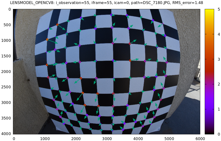
The residual vector for each chessboard corner in this observation is shown, scaled by a factor of 100 for legibility (the actual errors are tiny!) The circle color also indicates the magnitude of the errors. The size of each circle represents the weight given to that point. The weight is reduced for points that were detected at a lower resolution by the chessboard detector. Points thrown out as outliers are not shown at all. Note that we're showing the measurements which are a weighted pixel error: high pixels errors may be reported as a low error if they had a low weight.

This is the worst-fitting image, so any data-gathering issues will show up in this plot. Zooming in at the worst point (easily identifiable by the color) will clearly show any motion blur or focus issues. Incorrectly-detected corners will be visible: they will be outliers or they will have a high error. Especially with lean models, the errors will be higher towards the edge of the imager: the lens models fit the worst there. There should be no discernible pattern to the errors. In a perfect world, these residuals will look like random samples. Out-of-sync camera observations would show up as a systematic error vectors pointing in one direction. And the corresponding out-of-sync image would display equal and opposite errors. Rolling shutter effects would show a more complex, but clearly non-random pattern. It is usually impossible to get clean-enough data to make all the patterns disappear, but these systematic errors are not represented by the noise model, so they will result in biases and overly-optimistic uncertainty reports.

Back to the sample image. In absolute terms, even this worst-fitting image fits really well. The RMS error of the errors in this image is 1.48 pixels. The residuals in this image look mostly reasonable. There is a bit of a pattern: errors point outwardly in the center, larger errors on the outside of the image, pointing mostly inward. This isn't clearly indicative of any specific problem, so there's nothing obvious to fix, so we move on.

One issue with lean models such as LENSMODEL_OPENCV8 is that the radial distortion is never quite right, especially as we move further and further away form the optical axis: this is the last point in the common-errors list above. We can clearly see this here in the 3rd-worst image:

show_residuals_observation_worst(2, vectorscale = 100, circlescale=0.5,
                                 cbmax = 5.0)

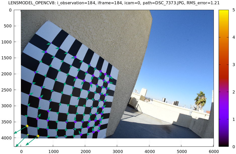
This is clearly a problem that should be addressed. Using a splined lens model instead of LENSMODEL_OPENCV8 makes this work, as seen in the tour of mrcal.

Another way to visualize the systematic errors in this solve is to examine the residuals over all observations, color-coded by their direction, ignoring the magnitudes:

show_residuals_directions(icam=0, unset='key')

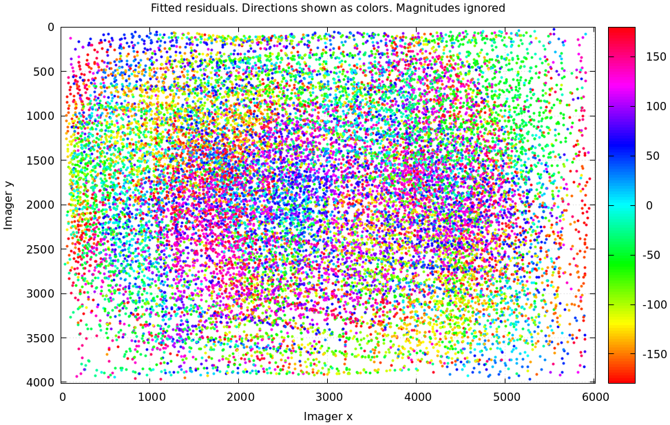
As before, if the model fit the observations, the errors would represent random noise, and no color pattern would be discernible in these dots. Here we can clearly see lots of green in the top-right and top and left, lots of blue and magenta in the center, yellow at the bottom, and so on. This is not random noise, and is a very clear indication that this lens model is not able to fit this data. To see what happens when a splined lens model is used for this data instead of LENSMODEL_OPENCV8, see the tour of mrcal.

It would be very nice to have a quantitative measure of these systematic patterns. At this time mrcal doesn't provide an automated way to do that.

Finally let's look at uncertainty reporting:

show_projection_uncertainty(icam=0)

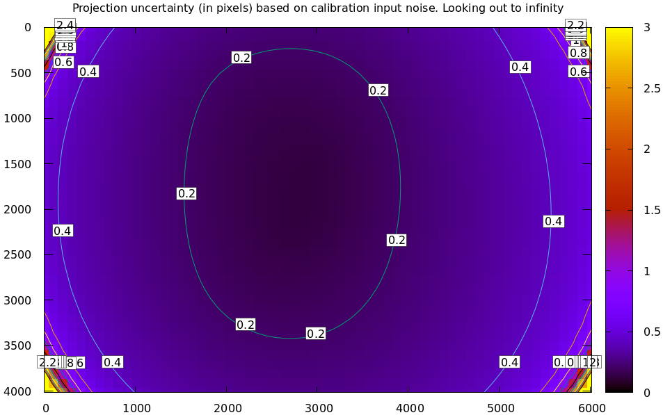
We could also have used the mrcal-show-projection-uncertainty tool from the shell. The uncertainties are shown as a color-map along with contours. These are the expected value of projection errors based on noise in input corner observations (given in --observed-pixel-uncertainty). By default, uncertainties for projection out to infinity are shown. If another distance is desired, pass that in the distance keyword argument. The lowest uncertainties are at roughly the range and imager locations of the the chessboard observations. Gaps in chessboard coverage will manifest as areas of high uncertainty (this is easier to see if we overlay the observations by passing the observations = True keyword argument).

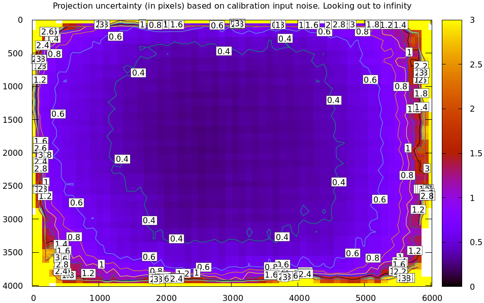
These uncertainty metrics are complementary to the residual metrics described above. If we have too little data, the residuals will be low, but the uncertainties will be very high. The more data we gather, the lower the uncertainties.

If the residual plots don't show any unexplained errors, then the uncertainty plots are the authoritative gauge of calibration quality. If the residuals do suggest problems, then the uncertainty predictions will be overly-optimistic: true errors will exceed the uncertainty predictions.

This applies when using lean models in general: the uncertainty reports assume the true lens is representable with the current lens model, so the stiffness of the lean lens models themselves will serve to decrease the reported uncertainty. For instance, the same uncertainty computed off the same data, but using a splined model (from the tour of mrcal):

Thus, if the residuals look reasonable, and the uncertainties look reasonable then we can use the resulting models, and hope to see the accuracy predicted by the uncertainty reports. Keep in mind that the value passed in --observed-pixel-uncertainty is usually a crude estimate, and it linearly affects the reported uncertainty values.