A tour of mrcal: triangulation

We just looked at dense stereo processing

This is an overview of a more detailed discussion about triangulation methods and uncertainty.

We just generated a range map: an image where each pixel encodes a range along each corresponding observation vector. This is computed relatively efficiently, but computing a range value for every pixel in the rectified image is still slow, and for many applications it isn't necessary. The mrcal triangulation routines take the opposite approach: given a discrete set of observed features, compute the position of just those features. In addition to being far faster, the triangulation routines propagate uncertainties and provide lots and lots of diagnostics to help debug incorrectly-reported ranges.

mrcal's sparse triangulation capabilities are provided by the mrcal-triangulate tool and the mrcal.triangulate() Python routine. Each of these ingests

• Some number of pairs of pixel observations \(\left\{ \vec q_{0_i}, \vec q_{1_i} \right\}\)
• The corresponding camera models
• The corresponding images

To produce

• The position of the point in space \(\vec p_i\) that produced these observations for each pair
• A covariance matrix, reporting the uncertainty of each reported point \(\Var\left( \vec p_i \right)\) and the covariances \(\Var \left( \vec p_i, \vec p_j \right)\)

Let's use our Downtown Los Angeles images. Before we start, one important caveat: there's only one camera, which was calibrated monocularly. The one camera was moved to capture the two images used to triangulate. The extrinsics were computed with a not-yet-in-mrcal tool, and mrcal cannot yet propagate the calibration noise in this scenario. Thus in this example we only propagate the observation-time noise.

Image from the left camera:

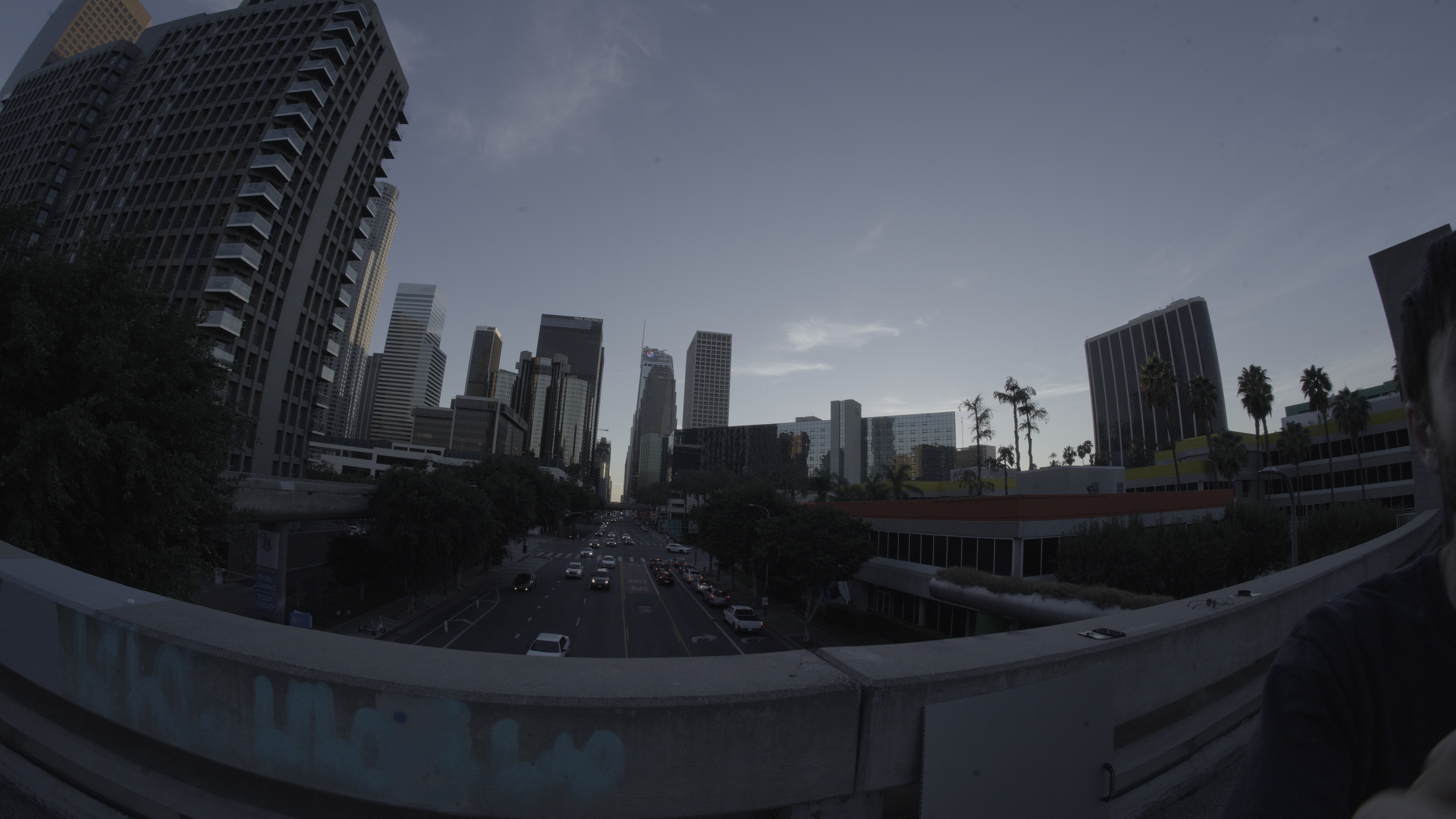
Let's compute the range to the top of the Wilshire Grand building, just as we did earlier.

The screenshot from mrcal-stereo --viz examined the pixel 2836.4,2045.7 in the rectified image. Let's convert it back to the out-of-the-left-camera image:

$ echo "2836.4 2045.7" |
  mrcal-reproject-points rectified0.cameramodel 0.cameramodel

2722.289377 1472.947733

Let's triangulate:

mrcal-triangulate                         \
    --range-estimate 873                  \
    --q-observation-stdev             0.3 \
    --q-observation-stdev-correlation 0.1 \
    --stabilize                           \
    --template-size 31 17                 \
    --search-radius 10                    \
    --viz uncertainty                     \
    [01].cameramodel                      \
    [01].jpg                              \
    2722.289377 1472.947733

Here we used the splined models computed earlier. We gave the tool the true range (873m) to use as a reference. And we gave it the expected observation noise level: 0.3 pixels (a loose estimate based on empirical experience). We declared the left-camera/right-camera pixel observations to be correlated with a factor of 0.1 on the stdev, so the relevant cross terms of the covariance matrix are \((0.3*0.1 \mathrm{pixels})^2\). It's not yet clear how to get the true value of this correlation, but we can use this tool to gauge its effects.

The mrcal-triangulate tool finds the corresponding feature in the second image using a template-match technique in mrcal.match_feature(). This operation could fail, so a diagnostic visualization can be requested by passing --viz match. This pops up an interactive window with the matched template overlaid in its best-fitting position so that a human can validate the match. The match was found correctly here. We could also pass --viz uncertainty, which shows the uncertainty ellipse. Unless we're looking very close in, this ellipse is almost always extremely long and extremely skinny. Here we have:

So looking at the ellipse usually isn't very useful, and the value printed in the statistics presents the same information in a more useful way. The mrcal-triangulate tool produces lots of reported statistics:

## Feature [2722.289 1472.948] in the left image corresponds to [2804.984 1489.036] at 873.0m
## Feature match found at [2805.443 1488.697]
## q1 - q1_perfect_at_range = [ 0.459 -0.339]
## Triangulated point at [ -94.251 -116.462  958.337]; direction: [-0.097 -0.12   0.988] [camera coordinates]
## Triangulated point at [-96.121 -81.23  961.719]; direction: [-0.097 -0.084  0.992] [reference coordinates]
## Range: 969.98 m (error: 96.98 m)
## q0 - q0_triangulation = [-0.023  0.17 ]
## Uncertainty propagation: observation-time noise suggests worst confidence of sigma=104.058m along [ 0.098  0.12  -0.988]
## Observed-pixel range sensitivity: 246.003m/pixel (q1). Worst direction: [0.998 0.07 ]. Linearized correction: -0.394 pixels
## Calibration yaw (rotation in epipolar plane) sensitivity: -8949.66m/deg. Linearized correction: 0.011 degrees of yaw
## Calibration yaw (cam0 y axis)                sensitivity: -8795.81m/deg. Linearized correction: 0.011 degrees of yaw
## Calibration pitch (tilt of epipolar plane) sensitivity: 779.47m/deg.
## Calibration translation sensitivity: 529.52m/m. Worst direction: [0.986 0.    0.165]. Linearized correction: -0.18 meters of translation
## Optimized yaw   (rotation in epipolar plane) correction = 0.012 degrees
## Optimized pitch (tilt of epipolar plane)     correction = 0.009 degrees
## Optimized relative yaw (1 <- 0): 0.444 degrees

We see that

• The range we compute here is 969.98m, not 873m as desired
• There's a difference of [-0.023 0.17] pixels between the triangulated point and the observation in the left camera: the epipolar lines are aligned well. This should be 0, ideally, but 0.17 pixels is easily explainable by pixel noise
• With the given observation noise, the 1-sigma uncertainty in the range is 104.058m, almost exactly in the observation direction. This is very similar to the actual error of 96.98m
• Moving the matched feature coordinate in the right image affects the range at worst at a rate of 246.003 m/pixel. Unsurprisingly, the most sensitive direction of motion is left/right. At this rate, it would take 0.394 pixels of motion to "fix" our range measurement
• Similarly, we compute and report the range sensitivity of extrinsic yaw (defined as the rotation in the epipolar plane or around the y axis of the left camera). In either case, an extrinsics yaw shift of 0.011 degrees would "fix" the range measurement.
• We also compute sensitivities for pitch and translation, but we don't expect those to affect the range very much, and we see that
• Finally, we reoptimize the extrinsics, and compute a better yaw correction to "fix" the range: 0.012 degrees. This is different from the previous value of 0.011 degrees because that computation used a linearized yaw-vs-range dependence, but the reoptimization doesn't.

This is all quite useful, and suggests that a small extrinsics error is likely the biggest problem.

What about --q-observation-stdev-correlation? What would be the effect of more or less correlation in our pixel observations? Running the same command with

• --q-observation-stdev-correlation 0 (the left and right pixel observations are independent) produces

  ## Uncertainty propagation: observation-time noise suggests worst confidence of sigma=104.580m along [ 0.098  0.12  -0.988]
  

• --q-observation-stdev-correlation 1 (the left and right pixel observations are perfectly coupled) produces

  ## Uncertainty propagation: observation-time noise suggests worst confidence of sigma=5.707m along [-0.095 -0.144  0.985]
  

I.e. correlations in the pixel measurements decrease our range uncertainty. To the point where perfectly-correlated observations produce almost perfect ranging. We'll still have range errors, but they would come from other sources than slightly mismatched feature observations.

A future update to mrcal will include a method to propagate uncertainty through to re-solved extrinsics and then to triangulation. That will fill-in the biggest missing piece in the error modeling here.