A tour of mrcal: stereo processing

We just found the best chessboard-dancing technique

This is an overview of a more detailed discussion about dense stereo.

We computed intrinsics from chessboards observations earlier, so let's use these for stereo processing.

I took several images off a catwalk over Figueroa Street in downtown Los Angeles. This is the view South along Figueroa Street. There're tall buildings ahead and on either side, which makes an interesting stereo scene.

The two images out of the camera look like this:

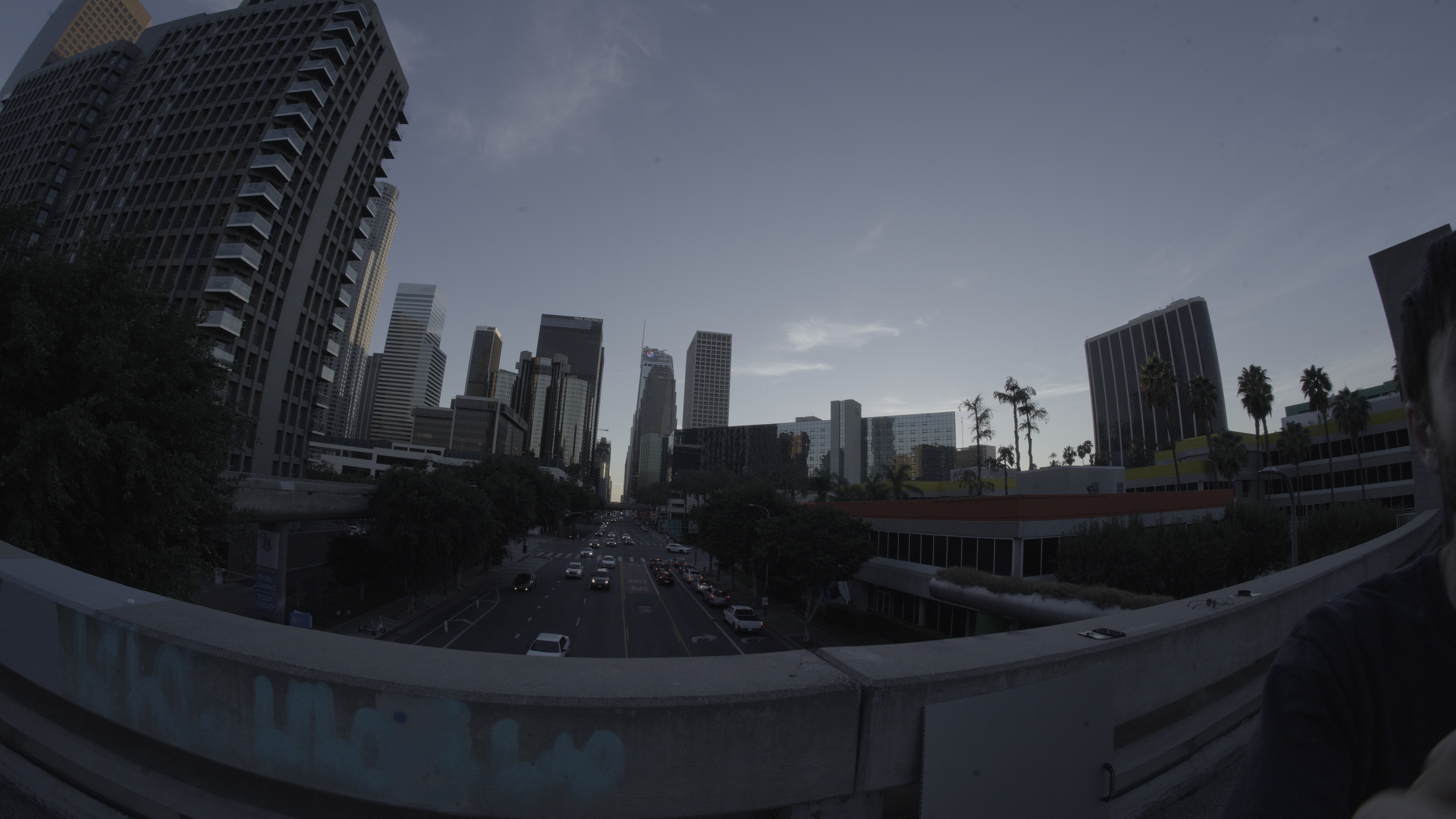
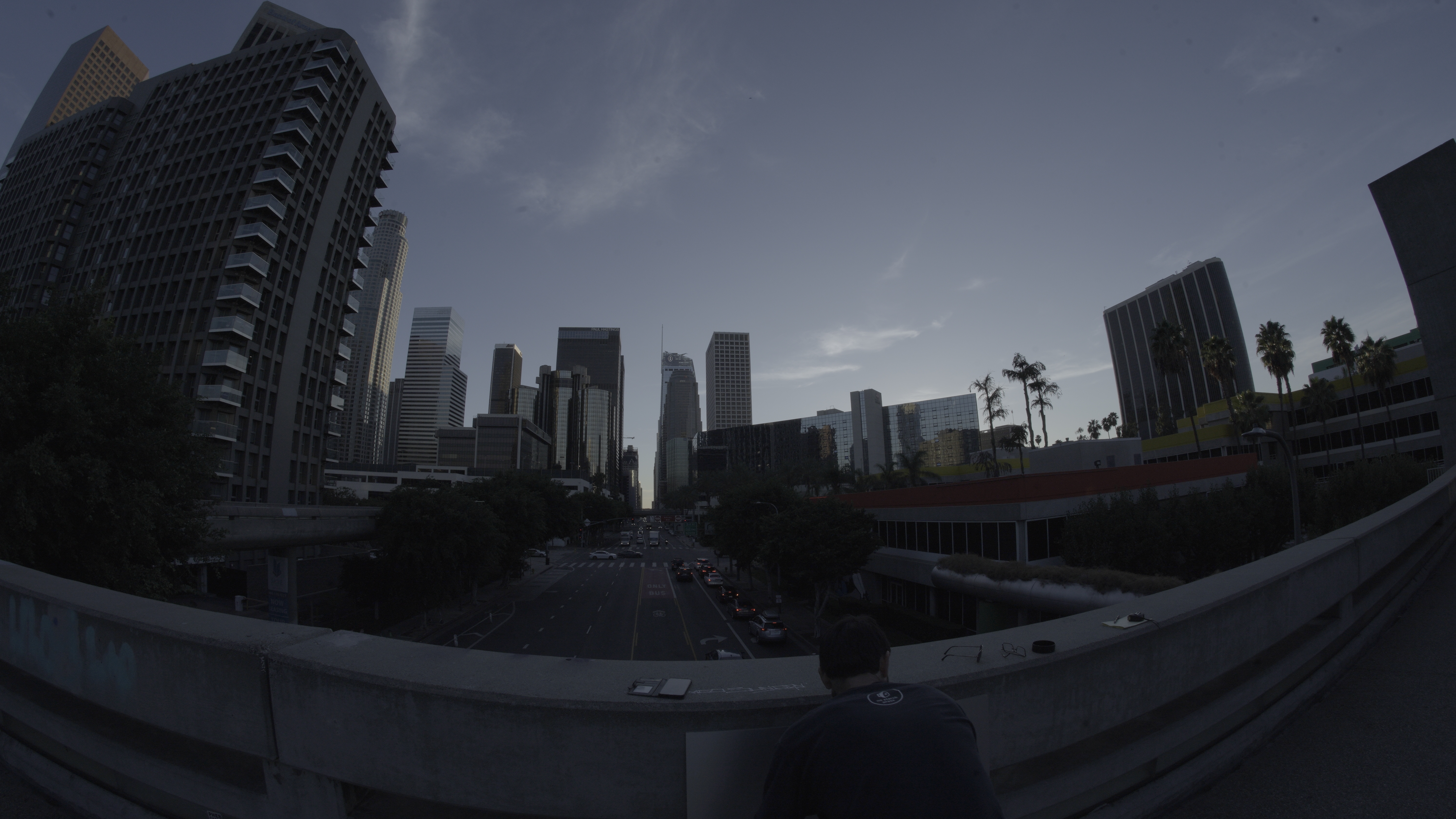
All the full-size images are available by clicking on an image.

The cameras are ~ 2m apart. In order to compute stereo images we need an accurate estimate of the relative geometry of the cameras, which we usually get as an output of the calibration process. Here I only had one physical camera, so I did something different:

• I calibrated the one camera monocularly, to get its intrinsics. This is what we computed thus far
• I used this camera to take a pair of images from slightly different locations. This is the "stereo pair"
• I used a separate tool to estimate the extrinsics from corresponding feature detections in the two images. For the purposes of this document the details of this don't matter

Generating a stereo pair in this way works well to demo the stereo processing tools. It does break the triangulation uncertainty reporting, since we lose the uncertainty information in the extrinsics, however. Preserving this uncertainty, and propagating it through the recomputed extrinsics to triangulation is on the mrcal roadmap. The resulting models we use for stereo processing:

• Left camera
• Right camera

I then use the mrcal-stereo tool to compute rectification maps, rectify the images, compute disparities and convert them to ranges:

mrcal-stereo                     \
  --az-fov-deg 170               \
  --az0-deg    10                \
  --el-fov-deg 95                \
  --el0-deg    -15               \
  --disparity-range 0 300        \
  --sgbm-p1 600                  \
  --sgbm-p2 2400                 \
  --sgbm-uniqueness-ratio 5      \
  --sgbm-disp12-max-diff  1      \
  --sgbm-speckle-window-size 100 \
  --sgbm-speckle-range 2         \
  --force-grayscale              \
  --clahe                        \
  [01].cameramodel               \
  [01].jpg                       \

The --sgbm-... options configure the OpenCV SGBM stereo matcher. Not specifying them uses the OpenCV defaults, which usually produces poor results.

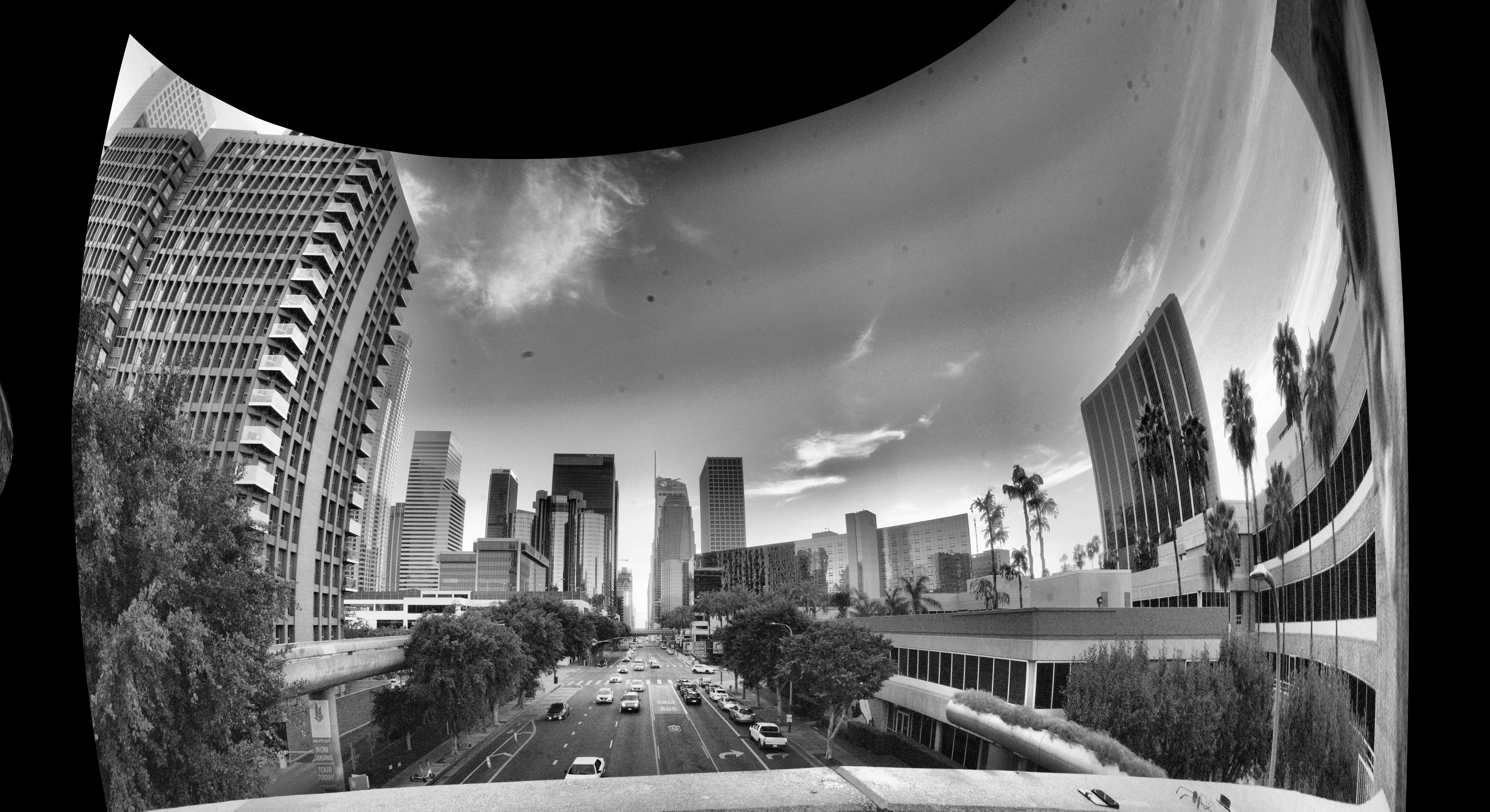
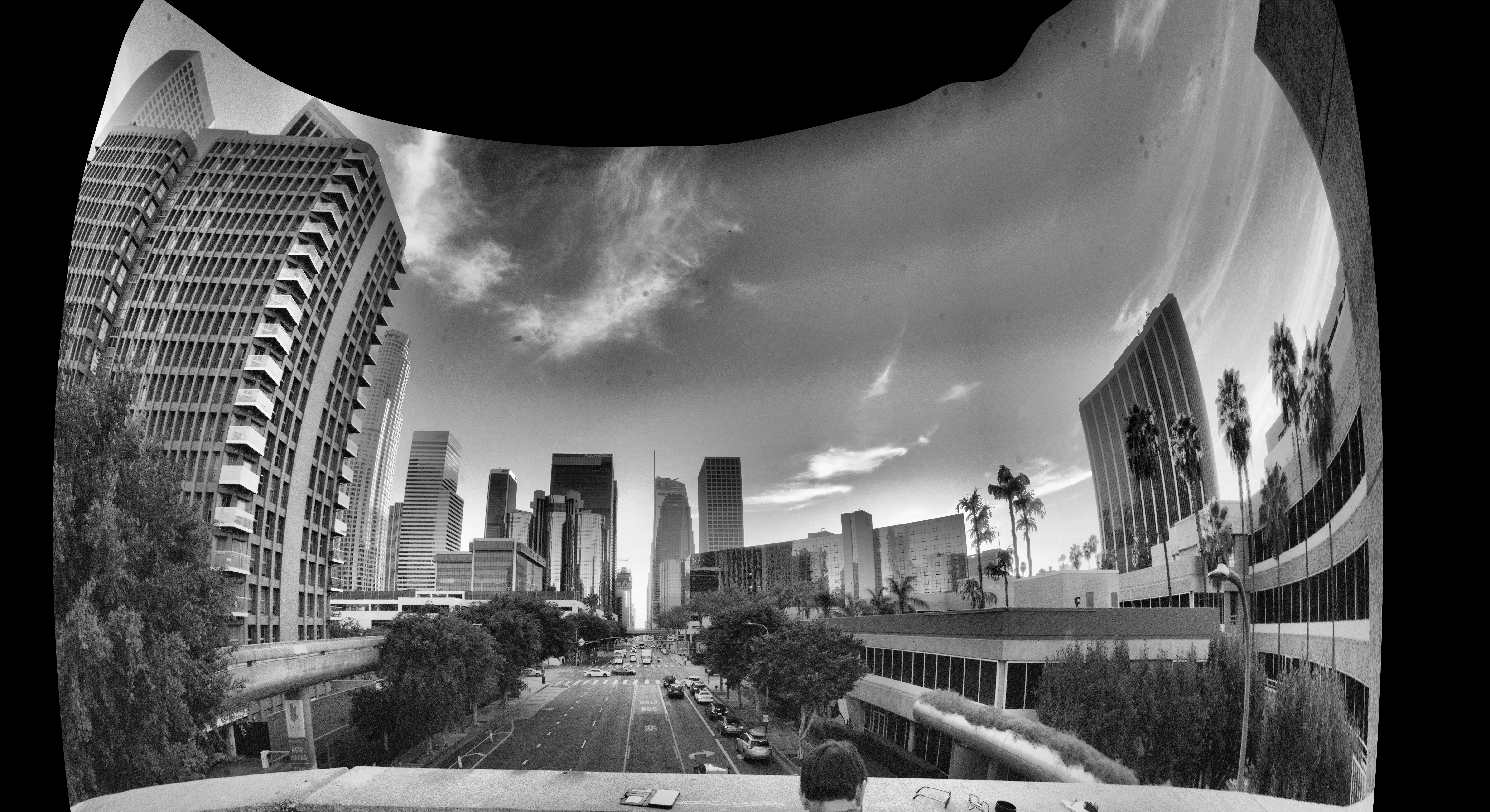
The rectified images look like this:

And the disparity and range images look like this:

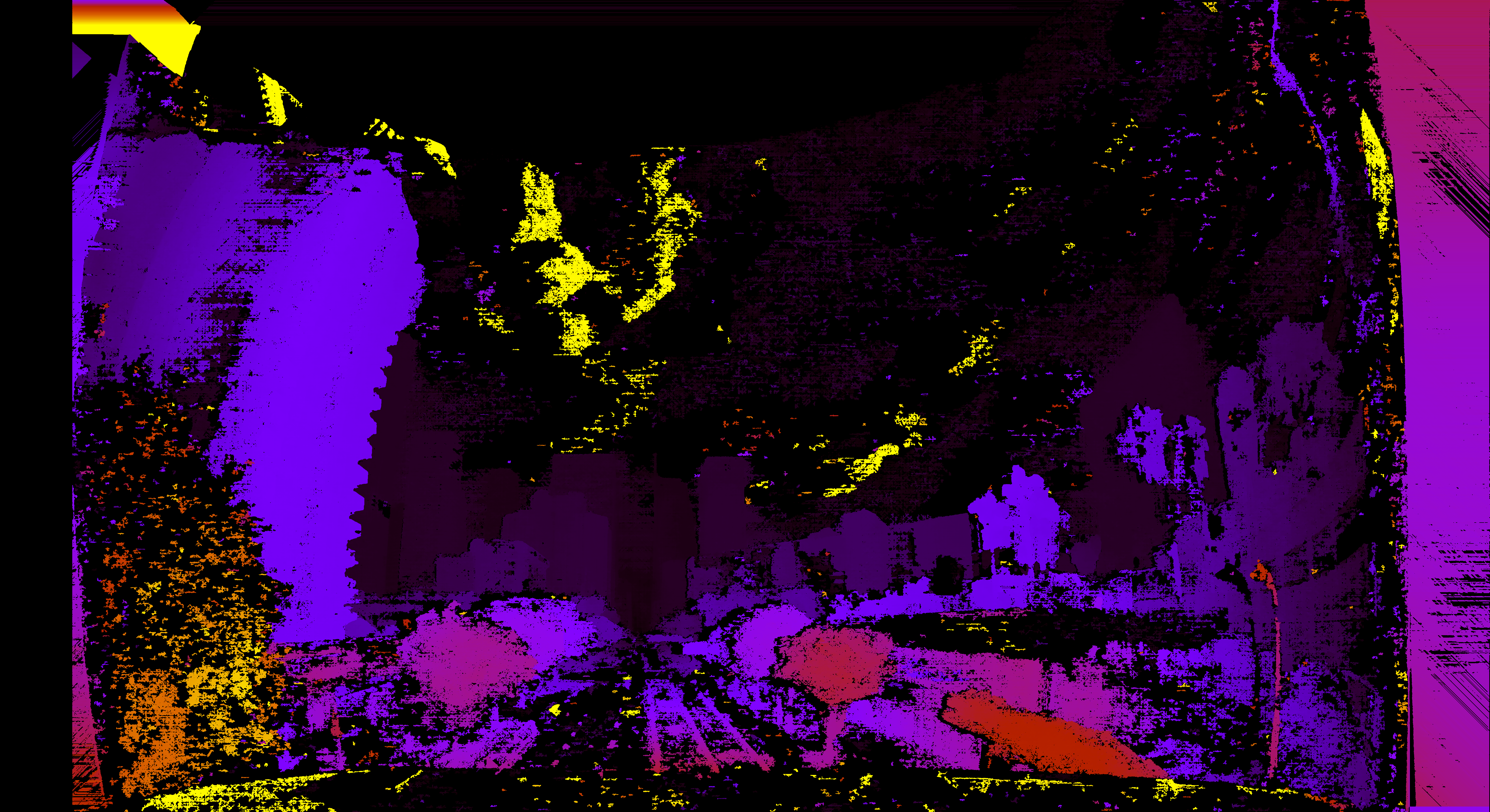
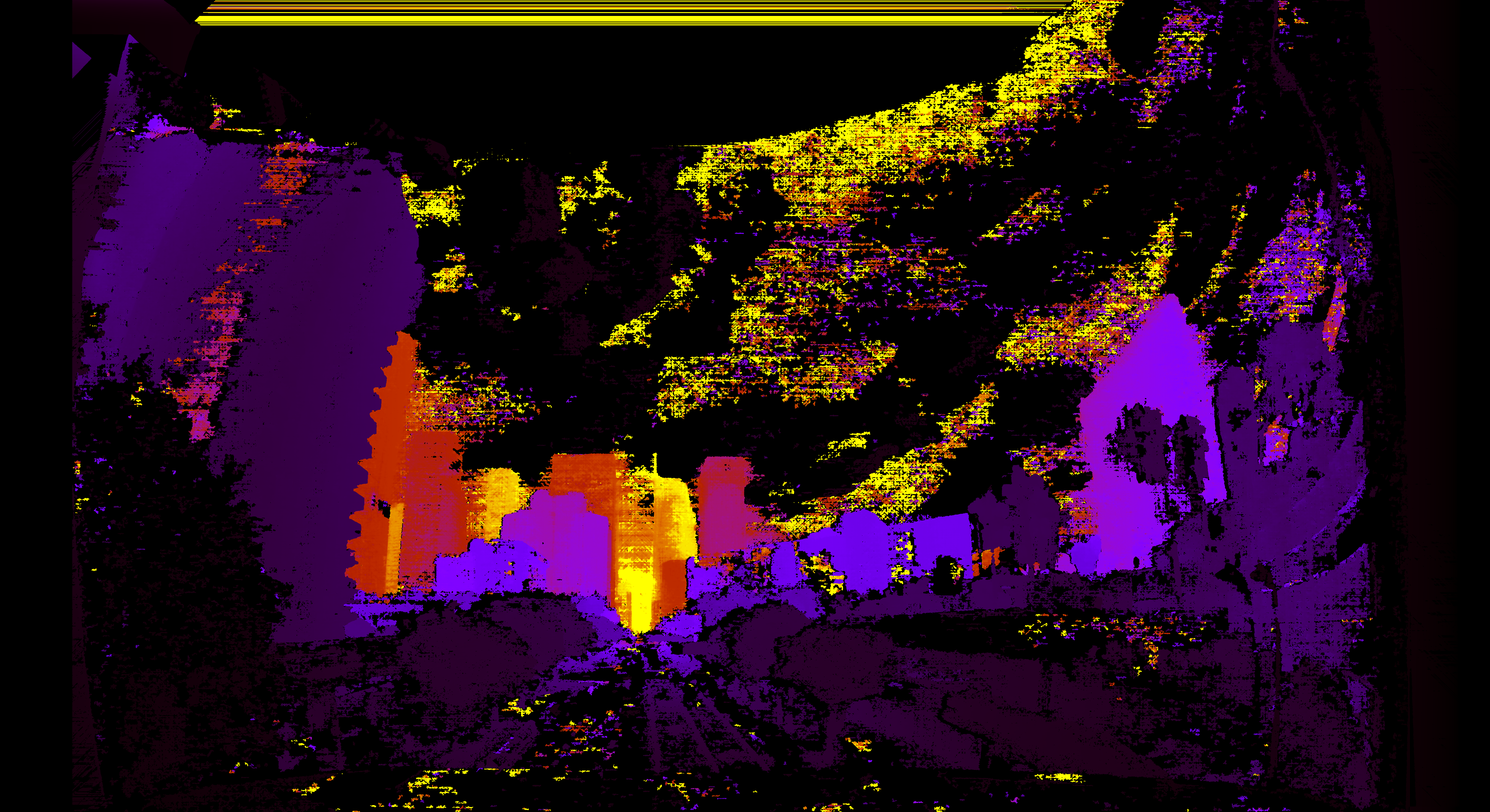
From a glance, this is clearly working well.

If you've used other stereo libraries previously, these rectified images may look odd: these are fisheye images, so the usual pinhole rectification would pull the corners out towards infinity. We don't see that here because mrcal-stereo uses the transverse equirectangular projection for rectification by default. This scheme samples the azimuth and elevation angles evenly, which minimizes the visual distortion inside each image row. Rectified models for this scene are generated by mrcal-stereo here and here. See the stereo-processing documentation for details.

The rectified models define a system with axes

• \(x\): the baseline; from the origin of the left camera to the origin of the right camera
• \(y\): down
• \(z\): forward

mrcal-stereo selects the \(y\) and \(z\) axes to line up as much as possible with the geometry of the input models. Since the geometry of the actual cameras may not match the idealized rectified geometry (the "forward" view direction may not be orthogonal to the baseline), the usual expectations that \(c_x \approx \frac{\mathrm{imagerwidth}}{2}\) and \(c_y \approx \frac{\mathrm{imagerheight}}{2}\) are not necessarily true in the rectified system. Thus it's valuable to visualize the models and the rectified field of view, for verification. mrcal-stereo can do that:

mrcal-stereo        \
  --az-fov-deg 170  \
  --az0-deg    10   \
  --el-fov-deg 95   \
  --el0-deg    -15  \
  --set 'view 70,5' \
  --viz geometry    \
  splined-[01].cameramodel

Here, the geometry is mostly nominal and the rectified view (indicated by the purple lines) does mostly lie along the \(z\) axis. This is a 3D plot that can be rotated by the user when mrcal-stereo --viz geometry is executed, making the geometry clearer.

The mrcal-stereo tool contains a visualizer that allows the user to quickly examine the stereo scene, evaluating the epipolar line alignment, disparities, ranges, etc. It can be invoked by runnung mrcal-stereo --viz stereo .... After panning/zooming, pressing r to display ranges (not disparities), and clicking on the Wilshire Grand building we get this:

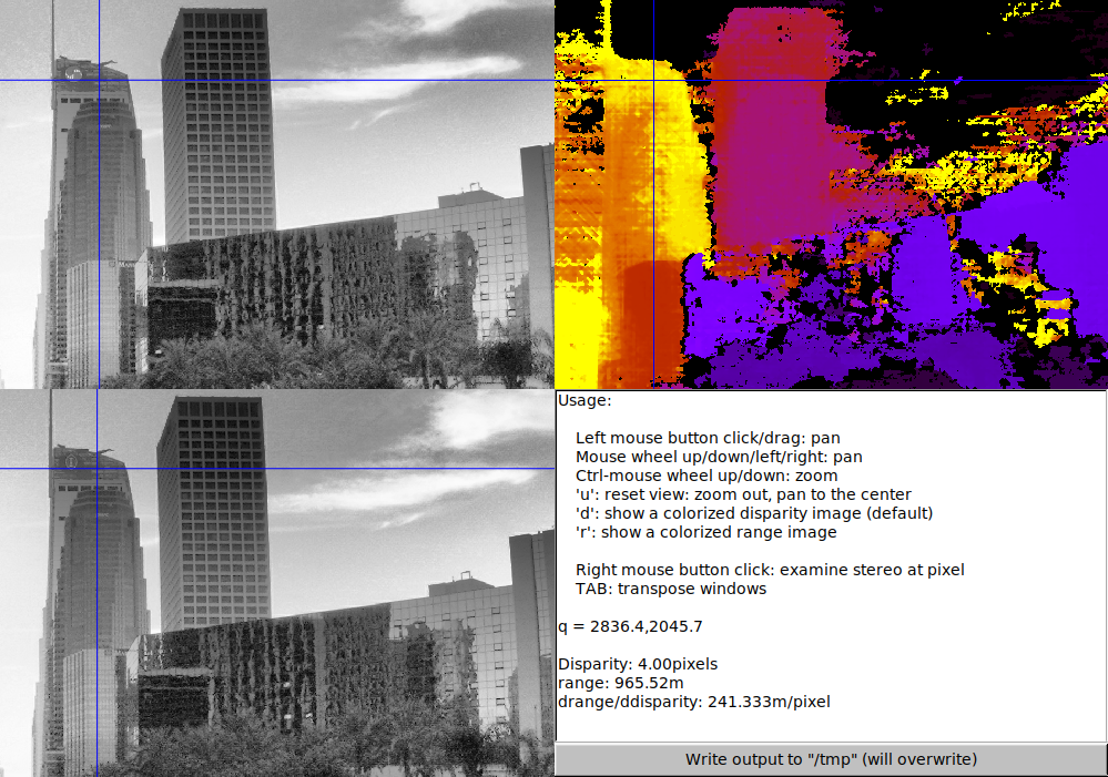
The computed range at that pixel is 965.52m. My estimated ground truth range is 873m. According to the linearized sensitivity reported by the tool, this corresponds to an error of \(\frac{966\mathrm{m}-873\mathrm{m}}{241.3\frac{\mathrm{m}}{\mathrm{pixel}}} = 0.39 \mathrm{pixels}\). Usually, stereo matching errors are in the 1/2 - 1/3 pixel range, so this is in-line with expectations.

Here we used dense stereo processing to compute a range map over the whole image. This is slow, and a lot of the time you can get away with computing ranges at a sparse set of points instead. So let's talk about triangulation routines.

We're ready to talk about triangulation routines