Model differencing
Table of Contents
mrcal provides a mrcal-show-projection-diff tool to compute and display the
projection differences between several models (implemented using
mrcal.show_projection_diff() and mrcal.projection_diff()). This has numerous
applications. For instance:
- evaluating the manufacturing variation of different lenses
- quantifying intrinsics drift due to mechanical or thermal stresses
- testing different solution methods
- underlying a cross-validation scheme
What is being computed?
What is meant by a "difference" here? Here we want to compare different representations of the same lens, so we're not interested in extrinsics. At a very high level, to evaluate the projection difference at a pixel coordinate \(\vec q_0\) in camera 0 we need to:
- Unproject \(\vec q_0\) to a fixed point \(\vec p\) using lens 0
- Project \(\vec p\) back to pixel coords \(\vec q_1\) using lens 1
- Report the reprojection difference \(\vec q_1 - \vec q_0\)

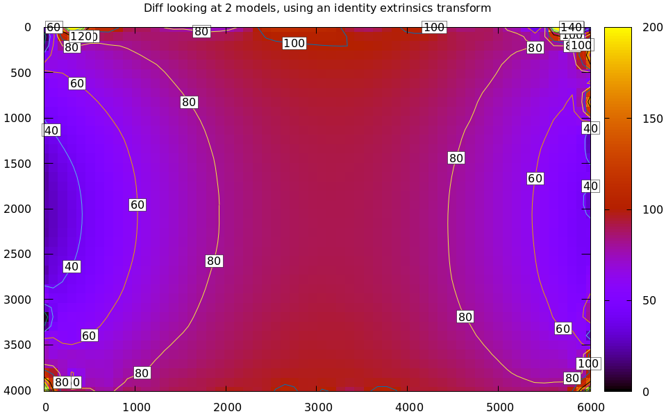
This simple definition is conceptually sound, but isn't applicable in practice. In the tour of mrcal, we calibrated the same lens using the same data, but with two different lens models. The models are describing the same lens, so we would expect a low difference. However, the above algorithm produces a difference that is very high. As a heat map:
mrcal-show-projection-diff \
  --intrinsics-only        \
  --cbmax 200              \
  --unset key              \
  opencv8.cameramodel      \
  splined.cameramodel
And as a vector field:
mrcal-show-projection-diff \
  --intrinsics-only        \
  --vectorfield            \
  --vectorscale 5          \
  --gridn 30 20            \
  --cbmax 200              \
  --unset key              \
  opencv8.cameramodel      \
  splined.cameramodel

The reported differences are in pixels.
The issue is similar to the one encountered by the projection uncertainty routine: each calibration produces noisy estimates of all the intrinsics and all the coordinate transformations:

The above plots projected the same \(\vec p\) in the camera coordinate system, but that coordinate system has shifted between the two models we're comparing. So in the fixed coordinate system attached to the camera housing, we weren't in fact projecting the same point.
There exists some transformation between the camera coordinate system from the solution and the coordinate system defined by the physical camera housing. It is important to note that this implied transformation is built-in to the intrinsics. Even if we're not explicitly optimizing the camera pose, this implied transformation is still something that exists and moves around in response to noise.
The above vector field suggests that we need to pitch one of the cameras. We can automate this by adding a critical missing step to the procedure above between steps 1 and 2:
- Transform \(\vec p\) from the coordinate system of one camera to the coordinate system of the other camera

We don't know anything about the physical coordinate system of either camera, so
we do the best we can: we compute a fit. The "right" transformation will
transform \(\vec p\) in such a way that the reported mismatches in \(\vec q\) will
be small. Previously we passed --intrinsics-only to bypass this fit. Let's
omit that option to get the the diff that we expect:
mrcal-show-projection-diff \
  --unset key              \
  opencv8.cameramodel      \
  splined.cameramodel
Implied transformation details
As with projection uncertainty, the difference computations are not invariant to range. So we always compute "the projection difference when looking out to \(r\) meters" for some possibly-infinite \(r\). The procedure we implement is:
- Regularly sample the two imagers, to get two corresponding sets of pixel coordinates \(\left\{\vec q_{0_i}\right\}\) and \(\left\{\vec q_{1_i}\right\}\)
- Unproject the camera-0 pixel coordinates to a set of points \(\left\{\vec
p_{0_i}\right\}\) in the camera-0 coordinate system. The range is given with
--distance.mrcal.sample_imager_unproject()function does this exactly - Compute corresponding unit observation vectors \(\left\{\vec v_{1_i}\right\}\) in the camera-1 coordinate system
- Compute the implied transformation \(\left(R,t\right)\) as the one to maximize
\[ \sum_i w_i \vec v_{1_i}^T \frac{R \vec p_{0_i} + t}{\left|R \vec p_{0_i} +
t\right|} \] where \(\left\{w_i\right\}\) is a set of weights. As with main
calibration optimization, this one is unconstrained, using the
rttransformation representation. The inner product above is \(\cos \theta\) where \(\theta\) is the angle between the two observation vectors.
When looking out to infinity the \(t\) becomes insignificant, and we do a rotation-only optimization.
This is the logic behind mrcal.implied_Rt10__from_unprojections() and
mrcal.projection_diff().
Selection of fitting data
The idea of using a fit to compute the implied transformation only works when the differences we're seeking are relatively small: once the \(\left(R,t\right)\) are found, the projection differences should be small, and all the fit residuals should be low. In many cases this is not a valid assumption. Example: we're comparing two calibrations of a wide lens, but one of the lens models is intended for a long lens, so it doesn't fit wide lenses well, and the projections agree only near the center. In this case, fitting observations everywhere in the imager will include poisoned data off center, and the optimal \(\left(R,t\right)\) will fit badly. And as a result, the reported diff will be high everywhere. However, if the dataset used for the fit is cut down to contain only observations near the center of the imager, then we will see the effect we expect: the two models would agree in the middle, and diverge at the edges.
Let's demonstrate this. I re-ran the calibration from the tour of mrcal using
LENSMODEL_OPENCV4. This model is not expected to work with wide lenses such as
this one. But the outlier rejection logic kicks in, makes the solve work as well
as it can:
$ mrcal-calibrate-cameras        \
  --corners-cache corners.vnl    \
  --lensmodel LENSMODEL_OPENCV4  \
  --focal 1700                   \
  --object-spacing 0.077         \
  --object-width-n 10            \
  --explore                      \
  '*.JPG'

vvvvvvvvvvvvvvvvvvvv initial solve: geometry only
^^^^^^^^^^^^^^^^^^^^ RMS error: 32.19393243308935

vvvvvvvvvvvvvvvvvvvv initial solve: geometry and intrinsic core only
^^^^^^^^^^^^^^^^^^^^ RMS error: 12.308083539621906
=================== optimizing everything except board warp from seeded intrinsics
mrcal.c(5042): Threw out some outliers (have a total of 491 now); going again
mrcal.c(5042): Threw out some outliers (have a total of 894 now); going again
..... a whole lot more of these
mrcal.c(5042): Threw out some outliers (have a total of 6764 now); going again
mrcal.c(5042): Threw out some outliers (have a total of 6801 now); going again
vvvvvvvvvvvvvvvvvvvv final, full re-optimization call to get board warp
mrcal.c(5042): Threw out some outliers (have a total of 6831 now); going again
^^^^^^^^^^^^^^^^^^^^ RMS error: 1.6712440499133436
RMS reprojection error: 1.7 pixels
Worst residual (by measurement): 8.7 pixels
Noutliers: 6831 out of 18600 total points: 36.7% of the data
calobject_warp = [-0.00115528  0.00043701]

Wrote ./camera-0.cameramodel
The resulting model is available here. This illustrates the differencing logic, but it isn't a good way to run calibrations in general: the outlier rejection will throw away the clearly-ill-fitting measurements, but marginal measurements will make it through, which will slightly poison the output.
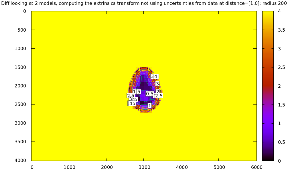
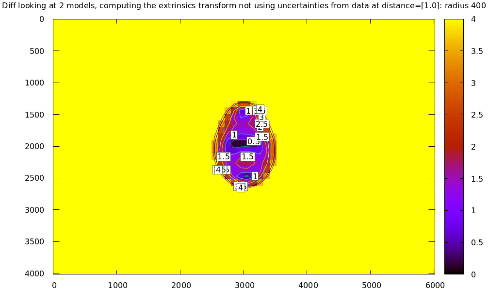
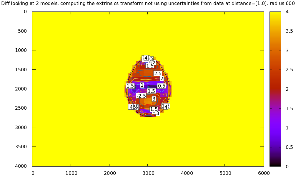
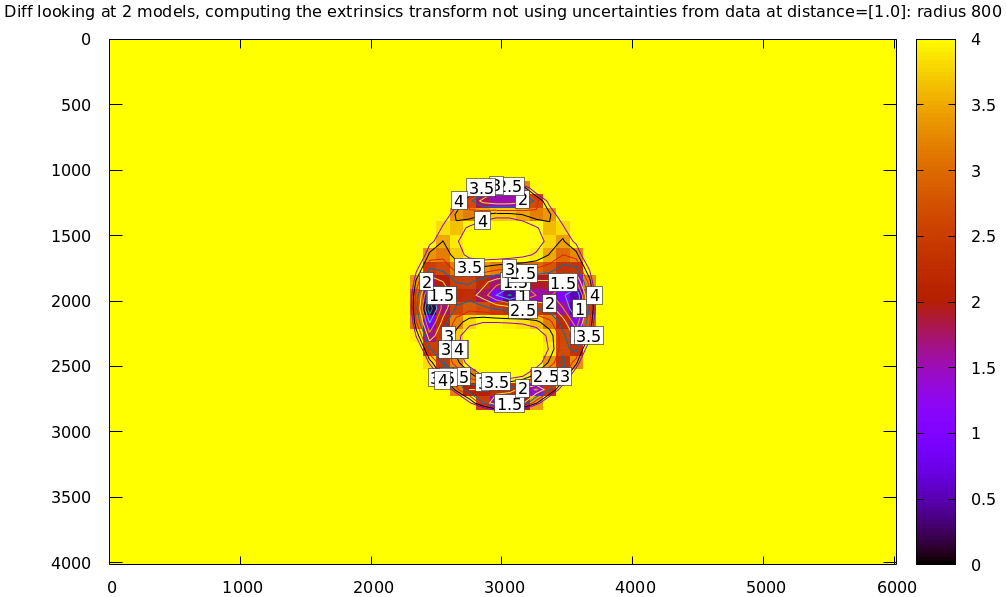
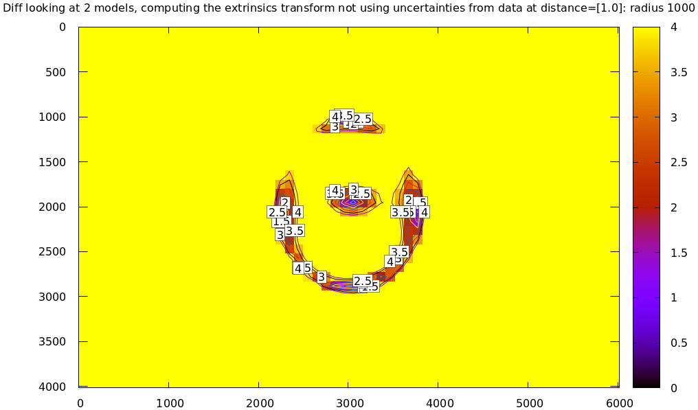
Let's compute the diff between the narrow-only LENSMODEL_OPENCV4 lens model
and the mostly-good-everywhere LENSMODEL_OPENCV8 model, using an expanding
radius of points. We expect this to work well when using a small radius, and we
expect the difference to degrade as we use more and more data away from the
center.
# This is a zsh loop
for r (200 400 600 800 1000) {
  mrcal-show-projection-diff \
    --no-uncertainties       \
    --distance 1             \
    --radius $r              \
    --unset key              \
    --extratitle "radius $r" \
    opencv[48].cameramodel
}
Fit weighting
Clearly the LENSMODEL_OPENCV4 solve does agree with the LENSMODEL_OPENCV8
solve well, but only in the center of the imager. The issue from a tooling
standpoint is that in order for the tool to tell us that, we needed to tell
the tool to only look at the center. That is not very useful.
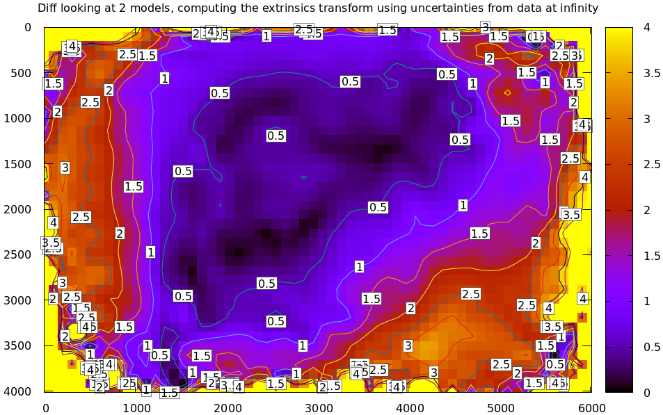
The issue we observed is that some regions of the imager have unreliable behavior, and poison the fit. But we know where the fit is reliable: in the areas where the projection uncertainty is low. So we can weigh the fit by the inverse of the projection uncertainty, and we will then automatically favor the "good" regions. Without requiring the user to specify the good-projection region.
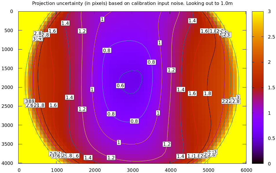
This works, but with a big caveat. As described on the projection uncertainty
page, lean models report overly-optimistic uncertainties. Thus when used as
weights for the fit, areas that actually are unreliable will be weighted too
highly, and will still poison the fit. We see that here, when comparing the
LENSMODEL_OPENCV4 and LENSMODEL_OPENCV8 results. The above plots show that
the LENSMODEL_OPENCV4 result is only reliable within a few 100s of pixels
around the center. However, LENSMODEL_OPENCV4 is a very lean model, so its
uncertainty at 1m out (near the sweet spot, where the chessboards were) looks
far better than that:
mrcal-show-projection-uncertainty \
    --distance 1                  \
    --unset key                   \
    opencv4.cameramodel
And the diff using that uncertainty as a weight without specifying a radius looks poor:
mrcal-show-projection-diff \
  --distance 1             \
  --unset key              \
  opencv[48].cameramodel
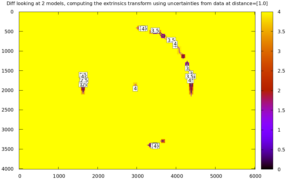
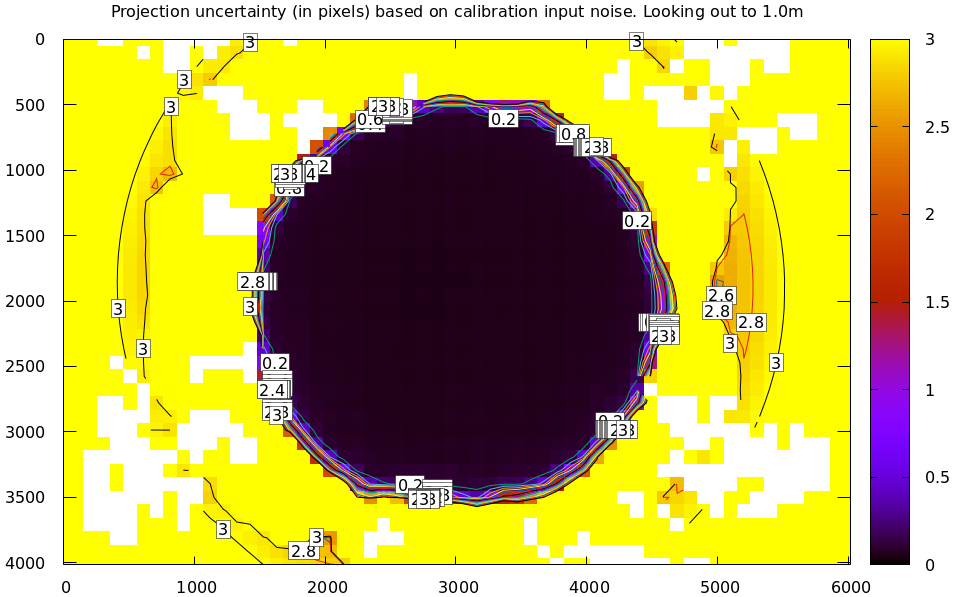
Where this technique does work well is when using splined models, which produce realistic uncertainty estimates. To demonstrate, let's produce a splined-model calibration that is only reliable in a particular region of the imager. We do this by culling the tour of mrcal calibration data to throw out all points outside of a circle at the center, calibrate off that data, and run a diff on those results:
< corners.vnl \
  mrcal-cull-corners --imagersize 6016 4016 --cull-rad-off-center 1500 \
> /tmp/raw.vnl &&
  vnl-join --vnl-sort - -j filename /tmp/raw.vnl \
     <(< /tmp/raw.vnl vnl-filter -p filename --has level |
                       vnl-uniq -c |
                       vnl-filter 'count > 20' -p filename ) \
  > corners-rad1500.vnl


mrcal-calibrate-cameras               \
  --corners-cache corners-rad1500.vnl \
  --lensmodel LENSMODEL_OPENCV4       \
  --focal 1700                        \
  --object-spacing 0.077              \
  --object-width-n 10                 \
  --explore                           \
  '*.JPG'

mrcal-show-projection-uncertainty \
  --distance 1                    \
  --unset key                     \
  splined-rad1500.cameramodel

mrcal-show-projection-diff \
  --distance 1             \
  --unset key              \
  splined{,-rad1500}.cameramodel
The cut-down corners are here and the resulting model is here. The uncertainty of this model looks like this:
and the diff like this:
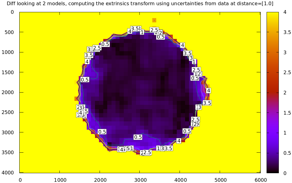
This is yet another reason to use only splined models for real-world lens modeling.