mrcal splined lens models
Table of Contents
mrcal supports a family of rich lens models to
- model real-world lens behavior with more fidelity than the usual parametric models make possible
- produce reliable projection uncertainty estimates
A summary of these models appears on the lens-model page:
LENSMODEL_SPLINED_STEREOGRAPHIC_... models, and we expand on it here.
The current approach is one of many possible ways to define a rich projection function based on splined surfaces. Improved representations could be developed in the future.
The idea of using a very rich representation to model lens behavior has been described in literature (for instance here and here). However, every paper I've seen models unprojection (mapping pixels to observation vectors) instead of projection (observation vectors to pixels). Projection is the usual direction, employed by every other lens model in every other toolkit, so following the papers would require rewriting lots and lots of code specifically to support this one model. mrcal's rich representation models projection, so this new model fits into the same framework as all the other models, and all the higher-level logic (differencing, uncertainty quantification, etc) continues to work with no changes.
Projection function
The LENSMODEL_SPLINED_STEREOGRAPHIC_... model is a stereographic model with
correction factors. To compute a projection using this model, we first compute
the normalized stereographic projection \(\vec u\) as in the
LENSMODEL_STEREOGRAPHIC definition:
\[ \theta \equiv \tan^{-1} \frac{\left| \vec p_{xy} \right|}{p_z} \]
\[ \vec u \equiv \frac{\vec p_{xy}}{\left| \vec p_{xy} \right|} 2 \tan\frac{\theta}{2} \]
Then we use \(\vec u\) to look-up a \(\Delta \vec u\) using two separate splined surfaces:
\[ \Delta \vec u \equiv \left[ \begin{aligned} \Delta u_x \left( \vec u \right) \\ \Delta u_y \left( \vec u \right) \end{aligned} \right] \]
and we then define the rest of the projection function:
\[\vec q = \left[ \begin{aligned} f_x \left( u_x + \Delta u_x \right) + c_x \\ f_y \left( u_y + \Delta u_y \right) + c_y \end{aligned} \right] \]
The \(\Delta \vec u\) are the off-stereographic terms. If \(\Delta \vec u = 0\), we get a plain stereographic projection.
The surfaces \(\Delta u_x\) and \(\Delta u_y\) are defined as B-splines, parametrized by the values of the "knots" (control points). These knots are arranged in a fixed grid in the space of \(\vec u\), with the grid density and extent set by the model configuration (i.e. not subject to optimization). The values at each knot are set in the intrinsics vector, and this controls the projection function.
B-spline details
We're using B-splines primarily for their local support properties: moving a knot only affects the surface in the immediate neighborhood of that knot. This makes our jacobian sparse, which is critical for rapid convergence of the optimization problem. Conversely, at any \(\vec u\), the sampled value of the spline depends only on the knots in the immediate neighborhood of \(\vec u\). A script used in the development of the splined model shows this effect:

We sampled a curve defined by two sets of cubic B-spline control points: they're the same except the one point in the center differs. We can see that the two spline-interpolated functions produce a different value only in the vicinity of the tweaked control point. And we can clearly see the radius of the effect: the sampled value of a cubic B-spline depends on the two control points on either side of the query point. A quadratic B-spline has a narrower effect: the sampled value depends on the nearest control point, and one neighboring control point on either side.
This plot shows a 1-dimension splined curve, but we have splined surfaces. To sample a spline surface:
- Arrange the control points in a grid
- Sample each row independently as a separate 1-dimensional B-spline
- Use these row samples as control points to sample the resulting column
Processing columns first and then rows produces the same result. The same dev script from above checks this.
Configuration
The configuration selects the LENSMODEL_SPLINED_STEREOGRAPHIC_... model
parameters that aren't subject to optimization. These define the high-level
behavior of the spline. We have:
order: the degree of each 1D polynomial. This is either 2 (quadratic splines, C1 continuous) or 3 (cubic splines, C2 continuous). At this time,3(cubic splines) is recommended. I haven't yet done a thorough study on this, but empirical results tell me that quadratic splines are noticeably less flexible, and require a denser spline to fit as well as a comparable cubic spline.NxandNy: The spline density. We have aNxbyNygrid of evenly-spaced control points. The ratio of this spline grid should be selected to match the aspect ratio of the imager. Inside each spline patch we effectively have a lean parametric model. Choosing a too-sparse spline spacing will result in larger patches, which aren't able to fit real-world lenses. Choosing a denser spacing results in more parameters and a more flexible model at the cost of needing more data and slower computations. No data-driven method of choosingNxorNyis available at this time, butNx=30_Ny=20appears to work well for some very wide lenses I tested with. An initial study of the effects of different spacings appears below.fov_x_deg: The horizontal field of view, in degrees. Selects the region in the space of \(\vec u\) where the spline is well-defined.fov_y_degis not included in the configuration: it is assumed proportional withNyandNx.fov_x_degis used to compute aknots_per_uquantity, and this is applied in both the horizontal and vertical directions.
Field-of-view selection
The few knots around any given \(\vec u\) define the value of the spline function there. These knots define "spline patch", a polynomial surface that fully represents the spline function in the neighborhood of \(\vec u\). As the sample point \(\vec u\) moves around, different spline patches, selected by a different set of knots are selected. With cubic splines, each spline patch is defined by the local 4x4 grid of knots (16 knots total). With quadratic splines, each spline is defined by a 3x3 grid.
Since the knots are defined on a fixed grid, it is possible to try to sample the spline beyond the region where the knots are defined (beyond our declared field of view). In this case we use the nearest spline patch, which could sit far away from \(\vec u\). So here we still use a 4x4 grid of knots to define the spline patch, but \(\vec u\) no longer sits in the middle of these knots: because we're past the edge, and the preferred knots aren't available.
This produces continuous projections everywhere, at the cost of reduced function
flexibility at the edges: the effective edge patches could be much larger that
the internal patches. We can control this by selecting a wide-enough fov_x_deg
to cover the full field-of-view of the camera. We then wouldn't be querying the
spline beyond the knots, since those regions in space are out-of-view of the
lens. fov_x_deg should be large enough to cover the field of view, but not so
wide to waste knots representing invisible space. It is recommended to estimate
this from the datasheet of the lens, and then to run a calibration. The
mrcal-show-splined-model-correction tool can then be used to compare the
valid-intrinsics region (area with sufficient calibration data) against the
bounds of the spline-in-bounds region.
Fidelity and uncertainties
This splined model has many more parameters, and is far more flexible than the lean parametric models (all the other currently-supported lens models). This has several significant effects.
These models are much more capable of representing the behavior of real-world
lenses than the lean models: at a certain level of precision the parametric
models are always wrong. The tour of mrcal shows a real-world fit using
LENSMODEL_OPENCV8 and a real-world fit using a splined model, where we can
clearly see that the splined model fits the data better.
The higher parameter counts do result in higher reported uncertainties (see the tour of mrcal for examples). This is a good thing: the lean models report uncertainty estimates that are low, but do not match reality. The higher uncertainty estimates from the splined models are truthful, however. This is because the uncertainty estimate algorithm constrains the lenses to the space that's representable by a given lens model, which is a constraint that only exists on paper. Since mrcal reports the covariance matrix of any projection operation, the uncertainty can be used to pass/fail a calibration or the covariance can be propagated to whatever is using the model.
It is thus recommended to use splined models even for long lenses, which do fit the pinhole model more or less.
Uncertainty wiggles
In the the tour of mrcal we evaluated the projection uncertainty of a splined-model solve:
mrcal-show-projection-uncertainty splined.cameramodel --cbmax 1 --unset key
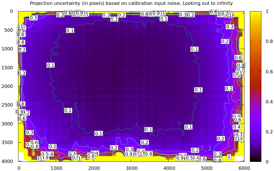
Note that the uncertainties from the splined model don't look smooth. Let's look into that now by evaluating the uncertainty across the imager at \(y = \frac{\mathrm{height}}{2}\). To do this we need to write a bit of Python code:
#!/usr/bin/python3
import mrcal
import numpy as np
import numpysane as nps
import gnuplotlib as gp
from scipy.signal import argrelextrema

m = mrcal.cameramodel('splined.cameramodel')
W,H = m.imagersize()

x = np.linspace(0, W-1, 1000)
q = np.ascontiguousarray( \
      nps.transpose(      \
        nps.cat(x, H/2*np.ones(x.shape))))

v = mrcal.unproject(q, *m.intrinsics())

s = mrcal.projection_uncertainty(v, m,
                                 atinfinity = True,
                                 what = 'worstdirection-stdev')
print(x[argrelextrema(s,np.greater)])

gp.plot(x, s,
        _with  = 'lines',
        xrange = (0,W-1),
        yrange = (0,0.2),
        xlabel = 'x pixel',
        ylabel = 'Projection uncertainty (pixels)',
        title  = 'Projection uncertainty at infinity, across the image at y=height/2')

We can clearly see the non-monotonicity. This feels like it has something to do with our spline knot layout, so let's check that. The above script also reports the \(x\) coordinates of the local maxima of the uncertainties:
array([ 258.9039039 ,  439.53453453,  638.22822823,  848.96396396,
       1059.6996997 , 1276.45645646, 1499.23423423, 1728.03303303,
       1950.81081081, 2179.60960961, 2414.42942943, 2649.24924925,
       2890.09009009, 3124.90990991, 3359.72972973, 3594.54954955,
       3829.36936937, 4064.18918919, 4292.98798799, 4509.74474474,
       4744.56456456, 4943.25825826, 5153.99399399, 5352.68768769,
       5846.41141141])
Let's look at the knot layout arbitrarily in the region near the center, marking the uncertainty maxima with red lines:
mrcal-show-splined-model-correction                                           \
  --imager-domain                                                             \
  --set 'xrange [2500:3500]'                                                  \
  --set 'yrange [1500:2500]'                                                  \
  --set 'arrow from 2649.3, graph 0 to 2649.3, graph 1 nohead lc "red" front' \
  --set 'arrow from 2890.1, graph 0 to 2890.1, graph 1 nohead lc "red" front' \
  --set 'arrow from 3124.9, graph 0 to 3124.9, graph 1 nohead lc "red" front' \
  --set 'arrow from 3359.7, graph 0 to 3359.7, graph 1 nohead lc "red" front' \
  --unset key                                                                 \
  splined.cameramodel
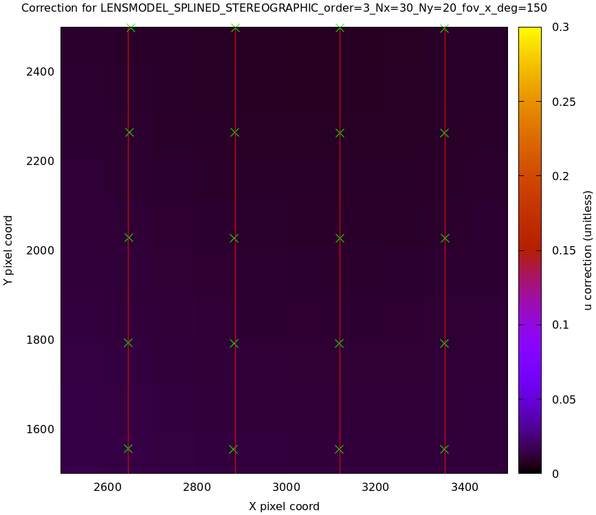
The uncertainty is clearly highest at the knots, so adjusting the spline spacing would have an effect here. I haven't yet studied the effect of changing the spline spacing, but we can do a quick study here. Let's re-run the splined model optimization in the the tour of mrcal, but using different spline spacings. And let's then reconstruct the uncertainty-across-center plot from above for each spacing.
We re-run the solves using this zsh script:
for Ny (4 6 8 10 15 20 25 30) {
  Nx=$((Ny*3/2))

  mrcal-calibrate-cameras                                                               \
    --corners-cache $D/data/board/corners.vnl                                           \
    --lensmodel LENSMODEL_SPLINED_STEREOGRAPHIC_order=3_Nx=${Nx}_Ny=${Ny}_fov_x_deg=150 \
    --focal 1700                                                                        \
    --object-spacing 0.077                                                              \
    --object-width-n 10                                                                 \
    --out /tmp/                                                                         \
    --imagersize 6016 4016                                                              \
    '*.JPG'

  mv /tmp/camera-0.cameramodel /tmp/splined-Nx=${Nx}-Ny=${Ny}.cameramodel
}
Results available here. And we write a bit of Python to make our plots:
#!/usr/bin/python3

import mrcal
import numpy as np
import numpysane as nps
import gnuplotlib as gp
import glob
import re

model_paths = np.array(glob.glob(f'splined-Nx=*.cameramodel'))

Nx = np.array([int(re.sub('.*Nx=([0-9]+).*?$', '\\1', p)) \
               for p in model_paths])
i = Nx.argsort()
model_paths = model_paths[i]

models = [mrcal.cameramodel(str(m)) for m in \
          model_paths]

W,H = models[0].imagersize()

x = np.linspace(0, W-1, 1000)
q = np.ascontiguousarray( \
      nps.transpose(      \
        nps.cat(x, H/2*np.ones(x.shape))))

s = np.array([mrcal.projection_uncertainty(mrcal.unproject(q, *m.intrinsics()),
                                           m,
                                           atinfinity = True,
                                           what = 'worstdirection-stdev') \
              for m in models])

legend = np.array([ re.sub('.*(Nx=[0-9]+)-(Ny=[0-9]+).*?$', '\\1 \\2', m) \
                    for m in model_paths ])

gp.plot(x, s,
        _with  = 'lines',
        legend = legend,
        xrange = (0,W-1),
        yrange = (0,0.2),
        xlabel = 'x pixel',
        ylabel = 'Projection uncertainty (pixels)',
        title  = 'Projection uncertainty at infinity, across the image at y=height/2',
        _set   = 'key bottom right',
        wait   = True)

So we can see that as we pick a denser spline:
- The uncertainty increases across the board. We already saw and noted this previously: lean models under-report the uncertainty
- The frequency of the uncertainty wiggle increases. This makes sense: we just noted that the wiggles follow the spline knots.
- The amplitude of the wiggle increases also. This is interesting. It could be due to the fact that a richer spline is better able to squeeze between the gaps between the observed points, or it could be a fundamental property of a B-spline. This needs a deeper investigation
Optimization practicalities
Core redundancy
As can be seen in the projection function above, the splined stereographic model parameters contain splined correction factors \(\Delta \vec u\) and an intrinsics core. The core variables are largely redundant with \(\Delta \vec u\): for any perturbation in the core, we can achieve a very similar change in projection behavior by bumping \(\Delta \vec u\) in a specific way. As a result, if we allow the optimization algorithm to control all the variables, the system will be under-determined, and the optimization routine will fail: complaining about a "not positive definite" (singular in this case) Hessian. At best the Hessian will be slightly non-singular, but convergence will be slow. To resolve this, the recommended sequence for optimizing splined stereographic models is:
- Fit the best
LENSMODEL_STEREOGRAPHICmodel to compute an estimate of the intrinsics core - Refine that solution with a full
LENSMODEL_SPLINED_STEREOGRAPHIC_...model, using the core we just computed, and asking the optimizer to lock down those core values. This can be done by setting thedo_optimize_intrinsics_corebit to 0 in themrcal_problem_selections_tstructure passed tomrcal_optimize()in C (or passingdo_optimize_intrinsics_core=Falsetomrcal.optimize()in Python).
This is what the mrcal-calibrate-cameras tool does.
Regularization
Another issue that comes up is the treatment of areas in the imager where no points were observed. By design, each parameter of the splined model controls projection from only a small area in space. So what happens to parameters controlling an area where no data was gathered? We have no data to suggest to the solver what values these parameters should take: they don't affect the cost function at all. Trying to optimize such a problem will result in a singular Hessian and complaints from the solver. We address this issue with regularization, to lightly pull all the \(\Delta \vec u\) terms to 0.
Another, related effect, is the interaction of extrinsics and intrinsics. Without special handling, splined stereographic solutions often produce a roll of the camera (rotation around the optical axis) to be compensated by a curl in the \(\Delta \vec u\) vector field. This isn't wrong per se, but is an unintended effect that's nice to eliminate. It looks really strange when a motion in the \(x\) direction in the camera coordinate system doesn't result in the projection moving in its \(x\) direction. We use regularization to handle this effect as well. Instead of pulling all the values of \(\Delta \vec u\) towards 0 evenly, we pull the \(\Delta \vec u\) acting tangentially much more than those acting radially. This asymmetry serves to eliminate any unnecessary curl in \(\Delta \vec u\).
Regardless of direction, these regularization terms are light. The weights are chosen to be small-enough to not noticeably affect the optimization in its fitting of the data. This may be handled differently in the future.
Uglyness at the edges
An unwelcome property of the projection function defined above, is that it allows aphysical, nonmonotonic behavior to be represented. For instance, let's look at the gradient in one particular direction.
\begin{aligned} q_x &= f_x \left( u_x + \Delta u_x \right) + c_x \\ \frac{\mathrm{d}q_x}{\mathrm{d}u_x} &\propto 1 + \frac{\mathrm{d}\Delta u_x}{\mathrm{d}u_x} \end{aligned}
We would expect \(\frac{\mathrm{d}q_x}{\mathrm{d}u_x}\) to always be positive, but
as we can see, here that depends on \(\frac{\mathrm{d}\Delta
u_x}{\mathrm{d}u_x}\), which could be anything since \(\Delta u_x\) is an
arbitrary splined function. Most of the time we're fitting the spline into real
data, so the real-world monotonic behavior will be represented. However, near
the edges quite often no data is available, so the behavior is driven by
regularization, and we're very likely to hit this non-monotonic behavior there.
This produces very alarming-looking spline surfaces, but it's not really a
problem: we get aphysical behavior in areas where we don't have data, so we have
no expectations of reliable projections there. The
mrcal-show-splined-model-correction tool visualizes either the bounds of the
valid-intrinsics region or the bounds of the imager. In many cases we have no
calibration data near the imager edges, so the spline is determined by
regularization in that area, and we get odd-looking knot layouts and imager
contours. A better regularization scheme or (better yet) a better representation
would address this. See a tour of mrcal for examples.