Projection uncertainty

Estimating the input noise
Propagating input noise to the state vector
Propagating the state vector noise through projection
Interfaces
The effect of range

After a calibration has been computed, it is essential to get a sense of how good the calibration is (how closely it represents reality). Traditional (non-mrcal) calibration routines rely on one metric of calibration quality: the residual fit error. This is clearly inadequate because we can always improve this metric by throwing away some input data, and it doesn't make sense that using less data would make a calibration better.

There are two main sources of error in the calibration solve. Without these errors, the calibration data would fit perfectly, producing a solve residual vector that's exactly \(\vec 0\). The two sources of error are:

Sampling error. Our computations are based on fitting a model to observations of chessboard corners. These observations aren't perfect, and contain a sample of some noise distribution. We can characterize this distribution and we can analytically predict the effects of that noise
Model error. These result when the solver's model of the world is insufficient to describe what is actually happening. When model errors are present, even the best set of parameters aren't able to completely fit the data. Some sources of model errors: motion blur, unsynchronized cameras, chessboard detector errors, too-simple (or unstable) lens models or chessboard deformation models, and so on. Since these errors are unmodeled (by definition), we can't analytically predict their effects. Instead we try hard to force these errors to zero, so that we can ignore them. We do this by using rich-enough models and by gathering clean data. To detect model errors we look at the solve diagnostics and we compute cross-validation diffs.

Let's do as much as we can analytically: let's gauge the effects of sampling error by computing a projection uncertainty for a model. Since only the sampling error is evaluated:

Any promises of a high-quality low-uncertainty calibration are valid only if the model errors are small.

The method to estimate the projection uncertainty is accessed via the mrcal.projection_uncertainty() function. Here the "uncertainty" is the sensitivity to sampling error: the calibration-time pixel noise. This tells us how good a calibration is (we aim for low projection uncertainties), and it can tell us how good the downstream results are as well (by propagating projection uncertainties through the downstream computation).

To estimate the projection uncertainty we:

Estimate the noise in the chessboard observations
Propagate that noise to the optimal parameters \(\vec b^*\) reported by the calibration routine
Propagate the uncertainty in calibration parameters \(\vec b^*\) through the projection function to get uncertainty in the resulting pixel coordinate \(\vec q\)

This overall approach is sound, but it implies some limitations:

Once again, model errors are not included in this uncertainty estimate
The choice of lens model affects the reported uncertainties. Lean models (those with few parameters) are less flexible than rich models, and don't fit general lenses as well as rich models do. This stiffness also serves to limit the model's response to noise in their parameters. Thus the above method will report less uncertainty for leaner models than rich models. So, unless we're sure that a given lens follows some particular lens model perfectly, a splined lens model (i.e. a very rich model) is recommended for truthful uncertainty reporting. Otherwise the reported confidence comes from the model itself, rather than the calibration data.

Estimating the input noise

We're measuring the sensitivity to the noise in the calibration-time observations. In order to propagate this noise, we need to know what that input noise is. The current approach is described in the optimization problem formulation.

Propagating input noise to the state vector

We solved the least squares problem, so we have the optimal state vector \(\vec b^*\).

We apply a perturbation to the input observations \(\vec q_\mathrm{ref}\), reoptimize this slightly-perturbed least-squares problem, assuming everything is linear, and look at what happens to the optimal state vector \(\vec b^*\).

We have

\[ E \equiv \left \Vert \vec x \right \Vert ^2 \] \[ J \equiv \frac{\partial \vec x}{\partial \vec b} \]

At the optimum \(E\) is minimized, so

\[ \frac{\partial E}{\partial \vec b} \left(\vec b = \vec b^* \right) = 2 J^T \vec x^* = 0 \]

We perturb the problem:

\[ E( \vec b + \Delta \vec b, \vec q_\mathrm{ref} + \Delta \vec q_\mathrm{ref})) \approx \left \Vert \vec x + \frac{\partial \vec x}{\partial \vec b} \Delta \vec b + \frac{\partial \vec x}{\partial \vec q_\mathrm{ref}} \Delta \vec q_\mathrm{ref} \right \Vert ^2 = \left \Vert \vec x + J \Delta \vec b + \frac{\partial \vec x}{\partial \vec q_\mathrm{ref}} \Delta \vec q_\mathrm{ref} \right \Vert ^2 \]

And we reoptimize:

\[ \frac{\mathrm{d}E}{\mathrm{d}\Delta \vec b} \approx 2 \left( \vec x + J \Delta \vec b + \frac{\partial \vec x}{\partial \vec q_\mathrm{ref}} {\Delta \vec q_\mathrm{ref}} \right)^T J = 0\]

We started at an optimum, so \(\vec x = \vec x^*\) and \(J^T \vec x^* = 0\), and thus

\[ J^T J \Delta \vec b = -J^T \frac{\partial \vec x}{\partial \vec q_\mathrm{ref}} {\Delta \vec q_\mathrm{ref}} \]

As defined on the input noise page, we have

\[ \vec x_\mathrm{observations} = W (\vec q - \vec q_\mathrm{ref}) \]

where \(W\) is a diagonal matrix of weights. These are the only elements of \(\vec x\) that depend on \(\vec q_\mathrm{ref}\). Let's assume the non-observation elements of \(\vec x\) are at the end, so

\[ \frac{\partial \vec x}{\partial \vec q_\mathrm{ref}} = \left[ \begin{array}{cc} - W \\ 0 \end{array} \right] \]

and thus

\[ J^T J \Delta \vec b = J_\mathrm{observations}^T W \Delta \vec q_\mathrm{ref} \]

So if we perturb the input observation vector \(q_\mathrm{ref}\) by \(\Delta q_\mathrm{ref}\), the resulting effect on the optimal parameters is \(\Delta \vec b = M \Delta \vec q_\mathrm{ref}\) where

\[ M = \left( J^T J \right)^{-1} J_\mathrm{observations}^T W \]

As usual,

\[ \mathrm{Var}\left(\vec b\right) = M \mathrm{Var}\left(\vec q_\mathrm{ref}\right) M^T \]

As stated on the input noise page, we're assuming independent noise on all observed pixels, with a standard deviation inversely proportional to the weight:

\[ \mathrm{Var}\left( \vec q_\mathrm{ref} \right) = \sigma^2 W^{-2} \]

\begin{aligned} \mathrm{Var}\left(\vec b\right) &= \sigma^2 M W^{-2} M^T \\ &= \sigma^2 \left( J^T J \right)^{-1} J_\mathrm{observations}^T W W^{-2} W J_\mathrm{observations} \left( J^T J \right)^{-1} \\ &= \sigma^2 \left( J^T J \right)^{-1} J_\mathrm{observations}^T J_\mathrm{observations} \left( J^T J \right)^{-1} \end{aligned}

If we have no regularization, then \(J_\mathrm{observations} = J\) and we can simplify even further:

\[\mathrm{Var}\left(\vec b\right) = \sigma^2 \left( J^T J \right)^{-1} \]

Note that these expressions do not explicitly depend on \(W\), but the weights still have an effect, since they are a part of \(J\). So if an observation \(i\) were to become less precise, \(w_i\) and \(x_i\) and \(J_i\) would all decrease. And as a result, \(\mathrm{Var}\left(\vec b\right)\) would increase, as expected.

Propagating the state vector noise through projection

We now have \(\mathrm{Var}\left(\vec b\right)\), and we can propagate this to evaluate the uncertainty of any component of the solve. Here I focus on the uncertainty of the intrinsics, since this is the biggest issue in most calibration tasks. So I propagate \(\mathrm{Var}\left(\vec b\right)\) through projection to get the projection uncertainty at any given pixel \(\vec q\). This is challenging because we reoptimize with each new sample of input noise \(\Delta \vec q_\mathrm{ref}\), and each optimization moves around all the coordinate systems:

Thus evaluating the projection uncertainty of \(\vec p_\mathrm{cam}\), a point in camera coordinates is not meaningful: the coordinate system itself moves with each re-optimization. Currently mrcal has multiple methods to address this:

the cross-reprojection uncertainty method: the new method available in mrcal 3.0. This is the preferred formulation
the mean-frames method: the simpler but somewhat problematic method used in earlier versions of mrcal

The goal of both of these methods is to compute a function \(\vec q^+\left(\vec b\right)\) to represent the change in projected pixel \(\vec q\) as the optimization vector \(\vec b\) moves around. If we have this function, then we can evaluate

\[ \mathrm{Var}\left( \vec q \right) = \frac{\partial \vec q^+}{\partial \vec b} \mathrm{Var}\left( \vec b \right) \frac{\partial \vec q^+}{\partial \vec b}^T \]

Interfaces

The mrcal.projection_uncertainty() function implements this logic. For the special-case of visualizing the uncertainties, call the any of the uncertainty visualization functions:

mrcal.show_projection_uncertainty(): Visualize the uncertainty in camera projection
mrcal.show_projection_uncertainty_vs_distance(): Visualize the uncertainty in camera projection along one observation ray

or use the mrcal-show-projection-uncertainty tool.

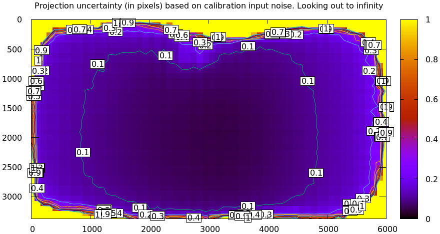
A sample uncertainty map of the splined model calibration from the tour of mrcal looking out to infinity:

mrcal-show-projection-uncertainty splined.cameramodel --cbmax 1 --unset key

The effect of range

We glossed over an important detail in the above derivation. Unlike a projection operation, an unprojection is ambiguous: given some camera-coordinate-system point \(\vec p\) that projects to a pixel \(\vec q\), we have \(\vec q = \mathrm{project}\left(k \vec v\right)\) for all \(k\). So an unprojection gives you a direction, but no range. The direct implication of this is that we can't ask for an "uncertainty at pixel coordinate \(\vec q\)". Rather we must ask about "uncertainty at pixel coordinate \(\vec q\) looking \(x\) meters out".

And a surprising consequence of that is that while projection is invariant to scaling (\(k \vec v\) projects to the same \(\vec q\) for any \(k\)), the uncertainty of projection is not invariant to this scaling:

Let's look at the projection uncertainty at the center of the imager at different ranges for an arbitrary model:

mrcal-show-projection-uncertainty \
  --vs-distance-at center         \
  --set 'yrange [0:0.1]'          \
  opencv8.cameramodel

So the uncertainty grows without bound as we approach the camera. As we move away, there's a sweet spot where we have maximum confidence. And as we move further out still, we approach some uncertainty asymptote at infinity. Qualitatively this is the figure I see 100% of the time, with the position of the minimum and of the asymptote varying.

As we approach the camera, the uncertainty is unbounded because we're looking at the projection of a fixed point into a camera whose position is uncertain. As we get closer to the origin, the noise in the camera position dominates the projection, and the uncertainty shoots to infinity.

The "sweet spot" where the uncertainty is lowest sits at the range where we observed the chessboards.

The uncertainty we asymptotically approach at infinity is set by the specifics of the chessboard dance.

See the tour of mrcal for a simulation validating this approach of quantifying uncertainty and for some empirical results.